Chapter 12 Assumptions

12.1 Learning Objectives

In this chapter we will review assumptions of MLMs and some ways to check them in R.

The learning objectives for this chapter are:

Understand the assumptions underpinning MLMs;
Develop and interpret R code and output for testing assumptions.

All materials for this chapter are available for download here.

12.2 Data Demonstration

12.2.1 Load Data and Dependencies

For this data demo, we will use the following packages:

library(lme4) # for multilevel models
library(lmerTest) # for p-values
library(dplyr) # for data manipulation
library(ggplot2) # for graphing

The data for chapter are a subsample from the 1982 High School Beyond data collected by the National Center for Educational Statistics, used as example data throughout Raudenbush, S. W., & Bryk, A. S. (2002). Hierarchical Linear Models: Applications and Data Analysis Methods: SAGE Publications. These data are related to student math achievement.

data <- read.csv('rb2002.csv')

12.2.2 Assumptions of MLMs

In brief, the assumptions underlying MLMs are as follows:

The model is correctly specified (i.e., all the predictors associated with the outcome and relevant random effects are included);
The functional form is correct (e.g., the relationship between the predictors and outcome is linear if using a linear model);
Level-1 residuals are independent and normally distributed;
Level-2 residuals are independent and multivariate normally distributed;
Residuals at level-1 and level-2 are unrelated;
Predictors at one level are not related to errors at another level (homoscedasticity).

In the data demonstration that follows, we will be showing some techniques for checking these assumptions. However, we note that there are many other ways to conduct similar checks. Assumption checks are data exploration at the end of the day. If you know and prefer other methods of exploring the same facets of your data, go for it!

12.2.3 Assumption 1: Model Specification

Specifying your model means determining which predictors should be included and what parameters to estimate. A correctly-specified model is one that includes everything associated with your outcome and nothing not-associated. This is impossible to know for certain and most researchers are constrained by the resources they have to get data and, ultimately, by the data they have. A general approach for considering this is trying to include all possible relevant IVs when predicting a DV. We recommend a three step approach. (1) Start with a null model to check the extent of clustering. (2) Run your “core” model, what you expect to be included according to theory. (3) Run a maximal model with all possible random effects, and trim down as you see effects are zero. Comparing models with and without effects and reviewing the literature for important variables to consider are decent strategies here. Get experts to read your results and their ideas on if anything is missing!

12.2.4 Assumption 2: Functional Form is Correct

The functional form of your model refers to the function connecting your predictors and outcome. In linear models like MLMs, that form is (you guessed it!) linear. However, you can use MLMs for non-linear data by specifying other functions, which are not covered in the current set of modules. In our example data, let’s look at the relationship between an outcome of math achievement (mathach) and a predictor of socioeconomic status (ses). We can get a sense of whether that relationship is linear with a scatterplot:

data %>% 
  ggplot(mapping = aes(x = ses, y = mathach)) +
  geom_point()

## Warning: Removed 1 rows containing missing values (geom_point).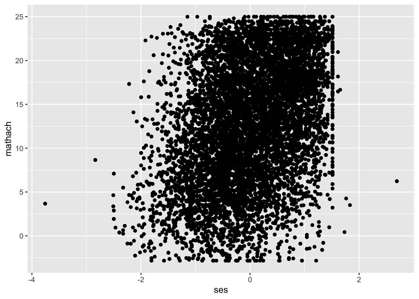

The scatterplot is hard to read because we have over 11,000 observations in our data. One option to improve readability is reducing the opacity of each point to get a clearer picture of how many points there are:

data %>% 
  ggplot(mapping = aes(x = ses, y = mathach)) +
  geom_point(alpha = .2)

## Warning: Removed 1 rows containing missing values (geom_point).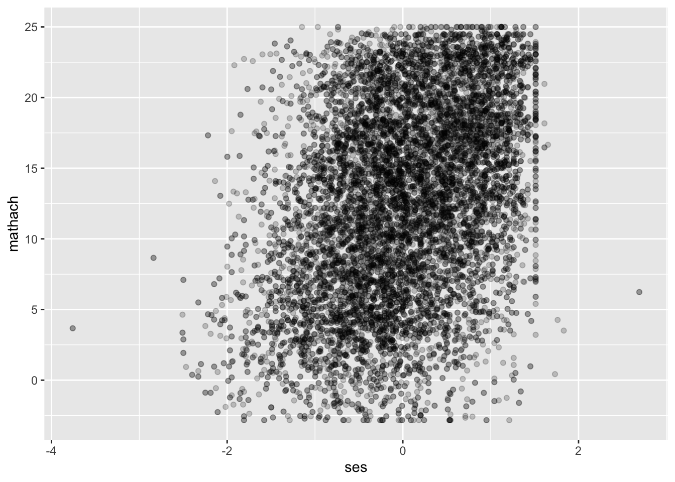

It looks loosely linear. Before we continue, for teaching purposes we’ll take a subset of 30 schools to make plotting easier for the rest of this data demo. For your data, you should consider all observations; this is just to make examples clearer.

data <- data %>%
    filter(SCHOOL %in% head(unique(SCHOOL), n = 30))

Let’s take a look at the relationship between SES and math achievement for each of the 30 schools in our subsetted data.

data %>% 
  ggplot() +
  geom_point(mapping = aes(x = ses, y = mathach)) +
  facet_wrap(~ SCHOOL)

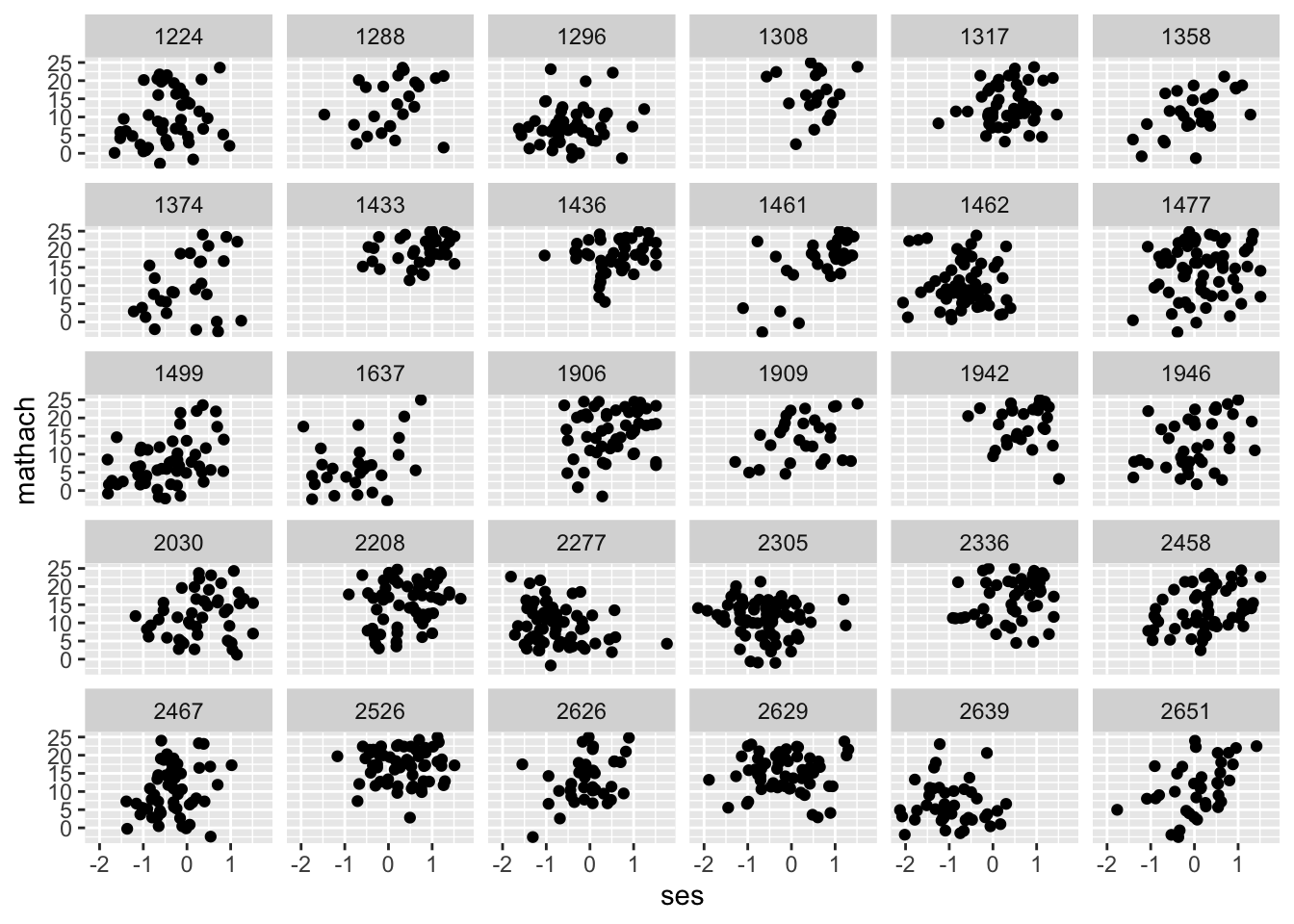
Looks like we have vaguely linear relationships; nothing looks quadratic. This is a subjective determination, be open to other, non-linear functions if a straight line doesn’t appear to do the job. Finally, let’s graph all points on one plane again but with regression lines overlaid for each school.

data %>% 
  group_by(SCHOOL) %>% 
  ggplot(mapping = aes(x = ses, y = mathach, colour = factor(SCHOOL))) +
  geom_point(show.legend = FALSE) +
  geom_smooth(method = lm, se = FALSE, show.legend = FALSE, fullrange = TRUE)

## `geom_smooth()` using formula 'y ~ x'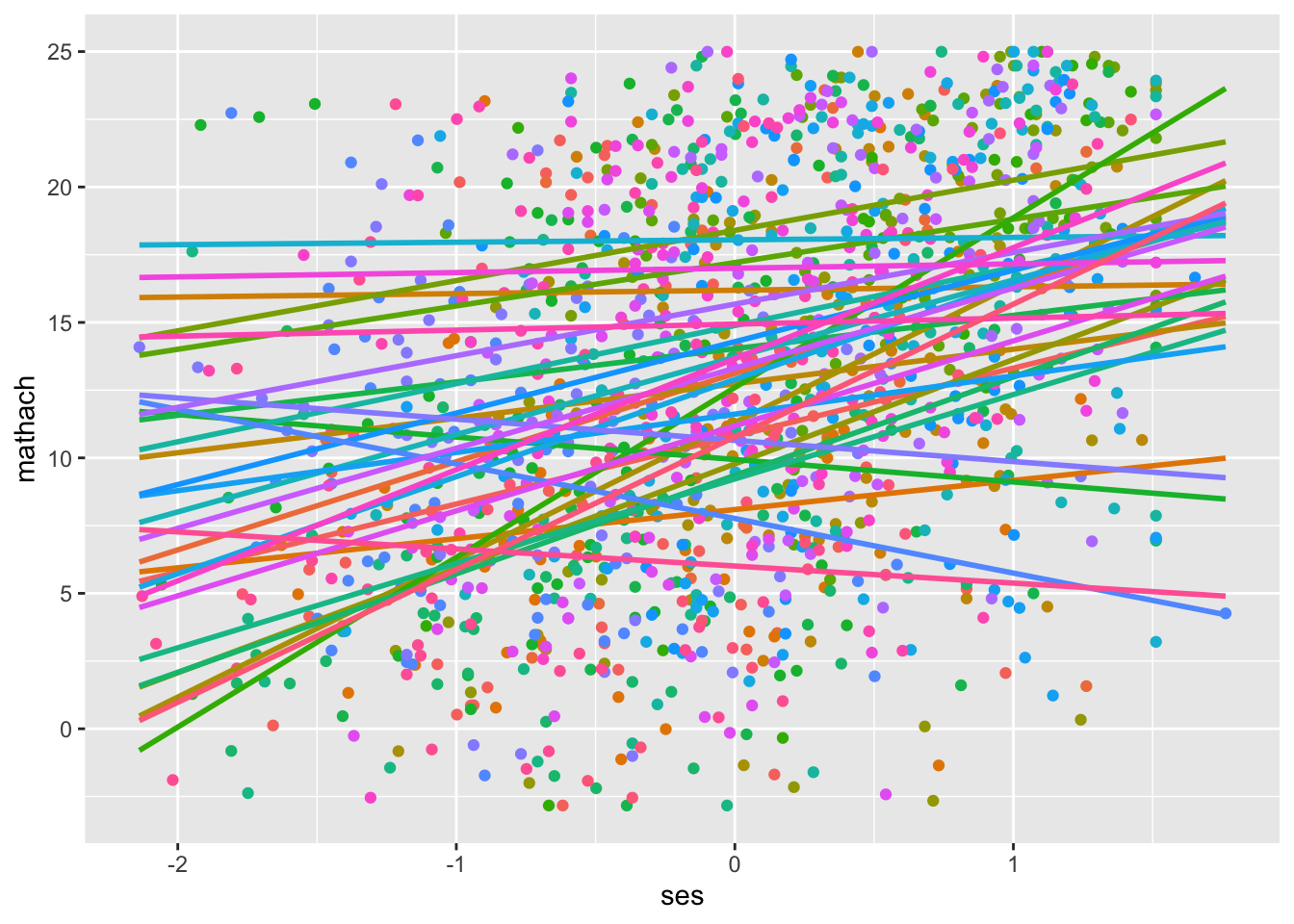

This isn’t an explicit test of functional form, but it looks like there is variance in intercepts and slopes across schools that merits multilevel modelling (or cluster-robust standard errors, if you don’t have any multilevel research questions).

12.2.5 An Aside: Extracting Residuals

In linear regression, we have the assumption of homoscedasticity. That is, the variance of residuals is roughly the same at any value of of your predictor(s). In multilevel models, we have two classes of residuals: level-1 residuals and level-2 residuals. The remaining assumptions all deal with these residuals: that they are normally distributed, that they don’t relate to each other, that they don’t relate to predictors at the same level or at the other level. We’re going to look at a model with math achievement predicted by SES centered within cluster (school) and mean SES predicting the intercept and slope of SES centered within cluster. We’ll estimate a random effect for the slope of SES centered within cluster. We’re not estimating the random effect covariance.

Level	Equation
Level 1	$mathach_{ij} = \beta_{0j} + \beta_{1j}cwc\_ses + R_{ij}$
Level 2	$\beta_{0j} = \gamma_{00} + \gamma_{10}ses\_mean + U_{0j}$
	$\beta_{1j} = \gamma_{10} + \gamma_{11}ses\_mean + U_{1j}$
Combined	$math_{ij} = \gamma_{00} + \gamma_{01}ses\_mean + \gamma_{10}cwc\_ses + \gamma_{11}cwc\_ses*ses\_mean + U_{0j} + U_{1j}cwc\_ses + R_{ij}$

model <- lmer(mathach ~  CWCses*ses_mean + (1|SCHOOL) + (0 + CWCses|SCHOOL), data = data, REML = TRUE)
summary(model)

## Linear mixed model fit by REML. t-tests use Satterthwaite's method ['lmerModLmerTest']
## Formula: mathach ~ CWCses * ses_mean + (1 | SCHOOL) + (0 + CWCses | SCHOOL)
##    Data: data
## 
## REML criterion at convergence: 8555.5
## 
## Scaled residuals: 
##      Min       1Q   Median       3Q      Max 
## -2.87105 -0.70607 -0.03647  0.76336  2.77351 
## 
## Random effects:
##  Groups   Name        Variance Std.Dev.
##  SCHOOL   (Intercept)  1.990   1.411   
##  SCHOOL.1 CWCses       1.379   1.174   
##  Residual             35.315   5.943   
## Number of obs: 1329, groups:  SCHOOL, 30
## 
## Fixed effects:
##                 Estimate Std. Error      df t value             Pr(>|t|)    
## (Intercept)      12.8243     0.3078 28.9279  41.661 < 0.0000000000000002 ***
## CWCses            1.9581     0.3412 27.3088   5.739      0.0000040499457 ***
## ses_mean          6.5269     0.6499 28.8676  10.044      0.0000000000628 ***
## CWCses:ses_mean   1.5239     0.7253 27.7253   2.101               0.0448 *  
## ---
## Signif. codes:  0 '***' 0.001 '**' 0.01 '*' 0.05 '.' 0.1 ' ' 1
## 
## Correlation of Fixed Effects:
##             (Intr) CWCses ses_mn
## CWCses       0.000              
## ses_mean    -0.026  0.000       
## CWCss:ss_mn  0.000  0.030  0.000

Let’s extract the level-1 residuals and add them to our data to work with moving forward:

data$l1resid <- residuals(model)
head(data$l1resid)

## [1] -1.9478535 10.1937749 10.7268788 -0.5893637  7.6105198 -6.0281684

We’ll extract the level-2 residuals shortly.

12.2.6 Assumption 3: Level-1 Residuals are Independent and Normally Distributed

12.2.6.1 Independent

Our level-1 residuals should be independent of our level-1 predictors. For our example, if our level-1 residuals ($\sigma^2$) correlate to SES centered within cluster, we have heteroscedasticity, which we don’t want. We can check this visually by creating a scatterplot of the predictor and the residuals:

data %>% 
  ggplot(mapping = aes(x = CWCses, y = l1resid)) +
  geom_point() +
  labs(x = "CWCses", y = "residuals")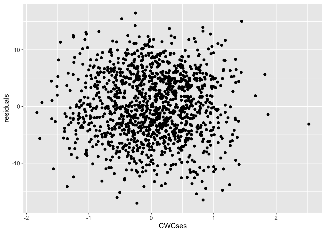

Those don’t look correlated; they look like a blob. We can check this statistically by calculating the correlation.

cor.test(data$l1resid, data$CWCses)

## 
##  Pearson's product-moment correlation
## 
## data:  data$l1resid and data$CWCses
## t = -0.0000000000000030409, df = 1327, p-value = 1
## alternative hypothesis: true correlation is not equal to 0
## 95 percent confidence interval:
##  -0.05377213  0.05377213
## sample estimates:
##                        cor 
## -0.00000000000000008347562

That correlation is essentially zero, meaning that our level-1 residuals and level-1 predictor are indeed uncorrelated!

12.2.6.2 Normally Distributed

We can check whether our level-1 residuals are normally distributed with a histogram:

data %>% 
  ggplot(mapping = aes(x = l1resid)) +
  geom_histogram()

## `stat_bin()` using `bins = 30`. Pick better value with `binwidth`.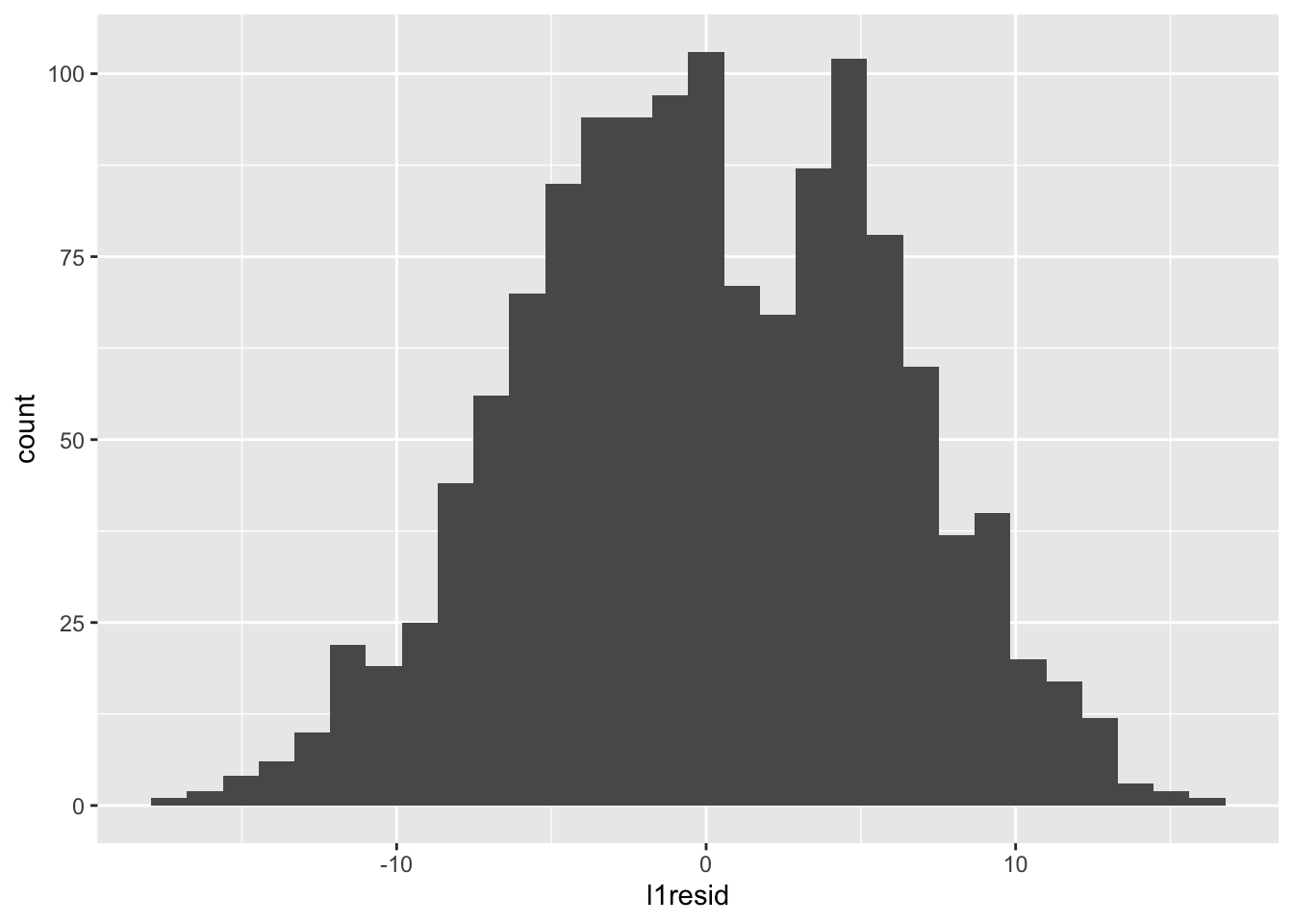

Those look normal-ish — there’s maybe something odd going on in that the distribution is bimodal, but that can be influenced by the number of bins. For example, with fewer bins:

data %>% 
  ggplot(mapping = aes(x = l1resid)) +
  geom_histogram(bins = 15)

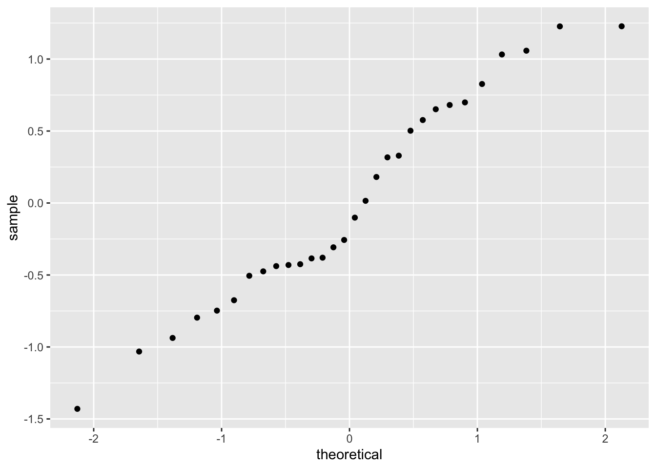
Let’s clear this up with a quantile-quantile (QQ) plot:

data %>% 
  ggplot(mapping = aes(sample = l1resid)) +
  stat_qq()

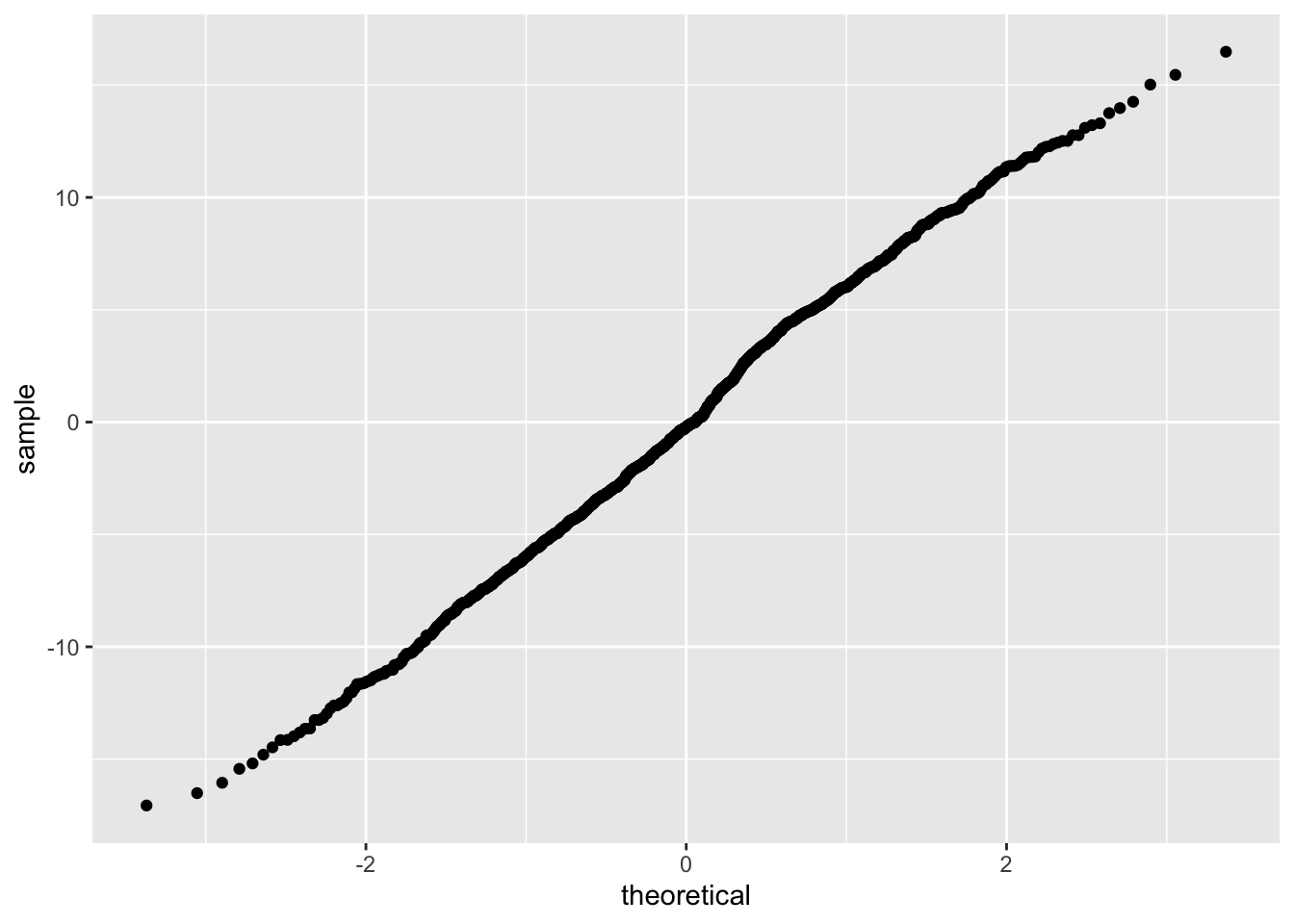
This plots quantiles for two distributions against each other: what proportion of points in our distribution is in a given quantile (y-axis), and how does that compare to the proportion of points in a given quantile for our theoretical normal distribution (x-axis). The line is straight, which indicates that our distribution is roughly normal.

12.2.7 Assumption 4: Level-2 Residuals are Independent and Multivariate Normal

To check our level-2 residual assumptions, we need to extract the level-2 residuals and add them to our data. This requires a little more work than extracting the level-1 residuals. We could easily add level-1 residuals to our dataset because every row is a person and had a residual. Level-2 residuals are at the school level, so the vector of residuals cannot be appended as easily. Let’s create a level-2 dataset to work with instead.

l2_data <- data %>% 
  group_by(SCHOOL) %>%  # group data by clustering variable, school
  mutate(
    mathach_mean = mean(mathach) # create mean math achievement per school
  ) %>% 
  select(SCHOOL, ses_mean, mathach_mean) %>% 
  unique() # select unique rows (rather than having school, ses_mean, and mathach_mean repeating over and over again)

Then let’s add the level-2 residuals to this dataset. We get two columns of residuals with the ranef(model)$SCHOOL command; the first column is intercept residuals $U_{0j}$s, the second column the slope residuals $U_{1j}$s. Matrices are indexed as [row, column], so we use the [, 1] code to get all rows from column 1 and [, 2] to get all rows from column 2.

l2_data$intercept_resid = ranef(model)$SCHOOL[, 1]
l2_data$slope_resid = ranef(model)$SCHOOL[, 2]

12.2.7.1 Independent

Like with level-1 residuals, we want our level-2 residuals to be independent from level-2 predictors. We also want both our level-2 residuals — intercept and slope residuals — to be independent of each other (which was not an issue at level-1, given that we only had one category of residual, $\sigma^2$). We can check whether our level-2 residuals are independent from the level-2 predictors and from one another as we did before: with a scatterplot and/or by calculating the correlation among them.

First, let’s look at the relationship between the intercept residuals and the level-2 variable of mean SES.

l2_data %>% 
  ggplot(mapping = aes(x = intercept_resid, y = ses_mean)) +
  geom_point()

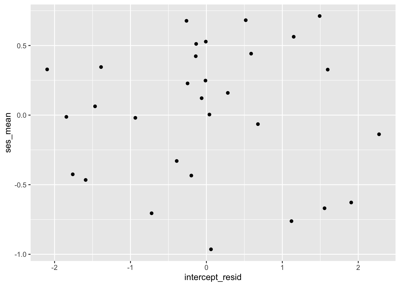And the correlation:

cor.test(l2_data$ses_mean, l2_data$intercept_resid)

## 
##  Pearson's product-moment correlation
## 
## data:  l2_data$ses_mean and l2_data$intercept_resid
## t = -0.000000000000077435, df = 28, p-value = 1
## alternative hypothesis: true correlation is not equal to 0
## 95 percent confidence interval:
##  -0.3602692  0.3602692
## sample estimates:
##                     cor 
## -0.00000000000001463377

Those look uncorrelated!

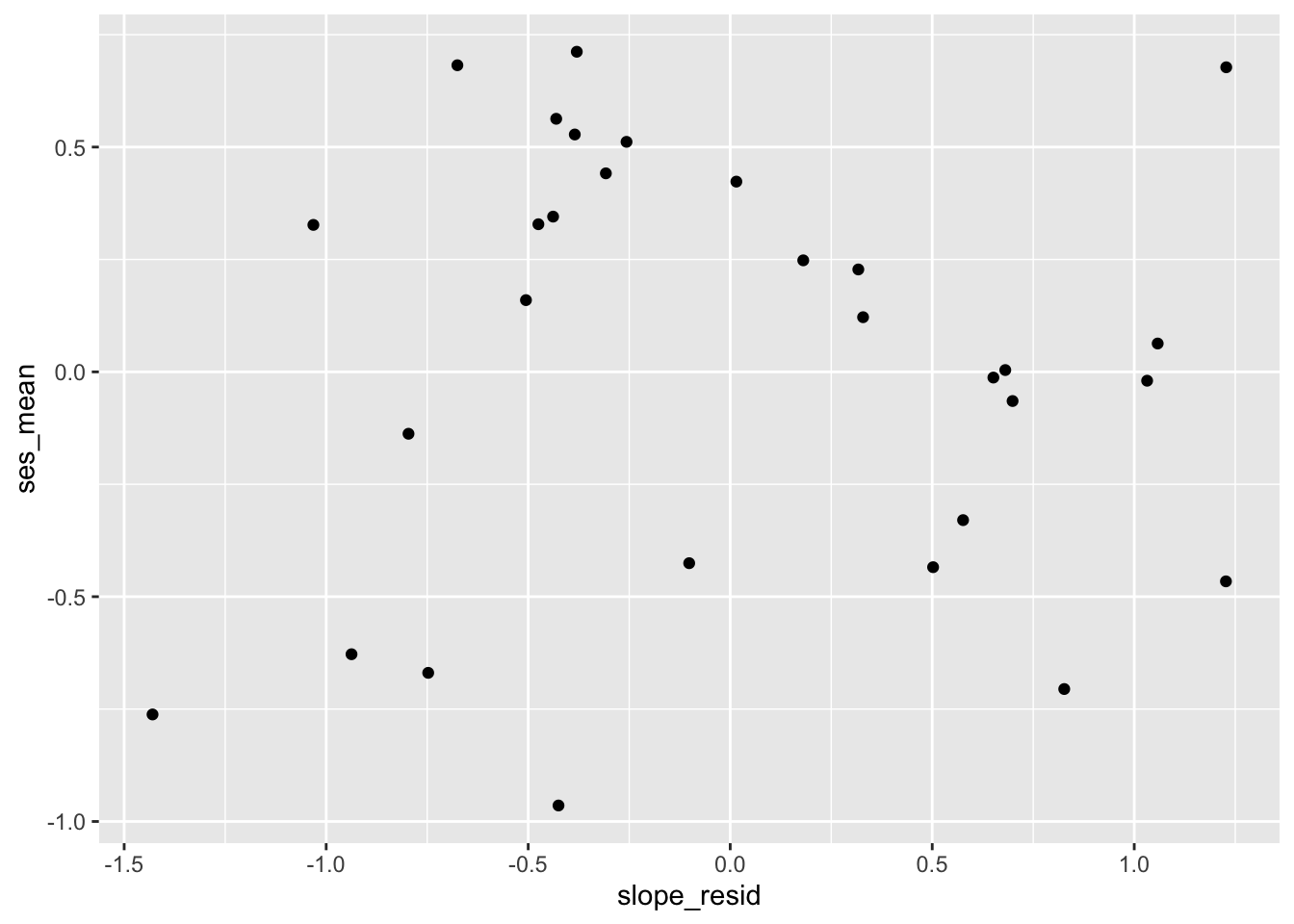
Next, let’s check that the slope residuals are independent from the predictor of mean SES:

l2_data %>% 
  ggplot(mapping = aes(x = slope_resid, y =ses_mean)) +
  geom_point()

cor.test(l2_data$ses_mean, l2_data$slope_resid)

## 
##  Pearson's product-moment correlation
## 
## data:  l2_data$ses_mean and l2_data$slope_resid
## t = 0.0000000000000036749, df = 28, p-value = 1
## alternative hypothesis: true correlation is not equal to 0
## 95 percent confidence interval:
##  -0.3602692  0.3602692
## sample estimates:
##                      cor 
## 0.0000000000000006944986

Those also look uncorrelated!

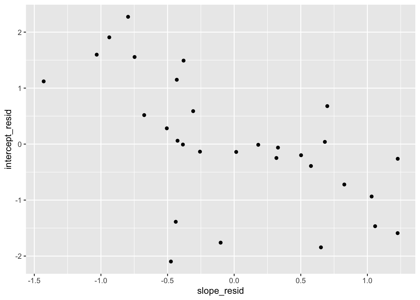
Finally, let’s check whether the level-2 residuals are independent of each other:

l2_data %>% 
  ggplot(mapping = aes(x = slope_resid, y = intercept_resid)) +
  geom_point()

cor.test(l2_data$intercept_resid, l2_data$slope_resid)

## 
##  Pearson's product-moment correlation
## 
## data:  l2_data$intercept_resid and l2_data$slope_resid
## t = -3.9046, df = 28, p-value = 0.0005424
## alternative hypothesis: true correlation is not equal to 0
## 95 percent confidence interval:
##  -0.7859072 -0.2970177
## sample estimates:
##        cor 
## -0.5937517

Our model assumes that intercept and slope residuals are independent, but that doesn’t seem to be the case. We could relax this by adding the covariance back in.

12.2.7.2 Multivariate Normal

As we did with our level-1 residuals, we can check the normality of our level-2 residuals with histograms and QQ plots. First, intercept residuals:

l2_data %>% 
  ggplot(mapping = aes(x = intercept_resid)) +
  geom_histogram(binwidth = .75)

l2_data %>% 
  ggplot(mapping = aes(sample = intercept_resid)) +
  stat_qq()

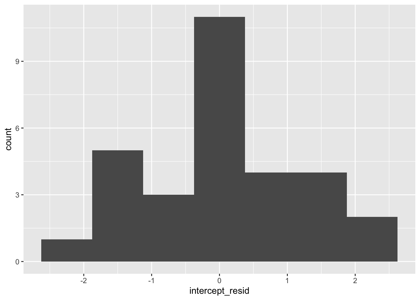
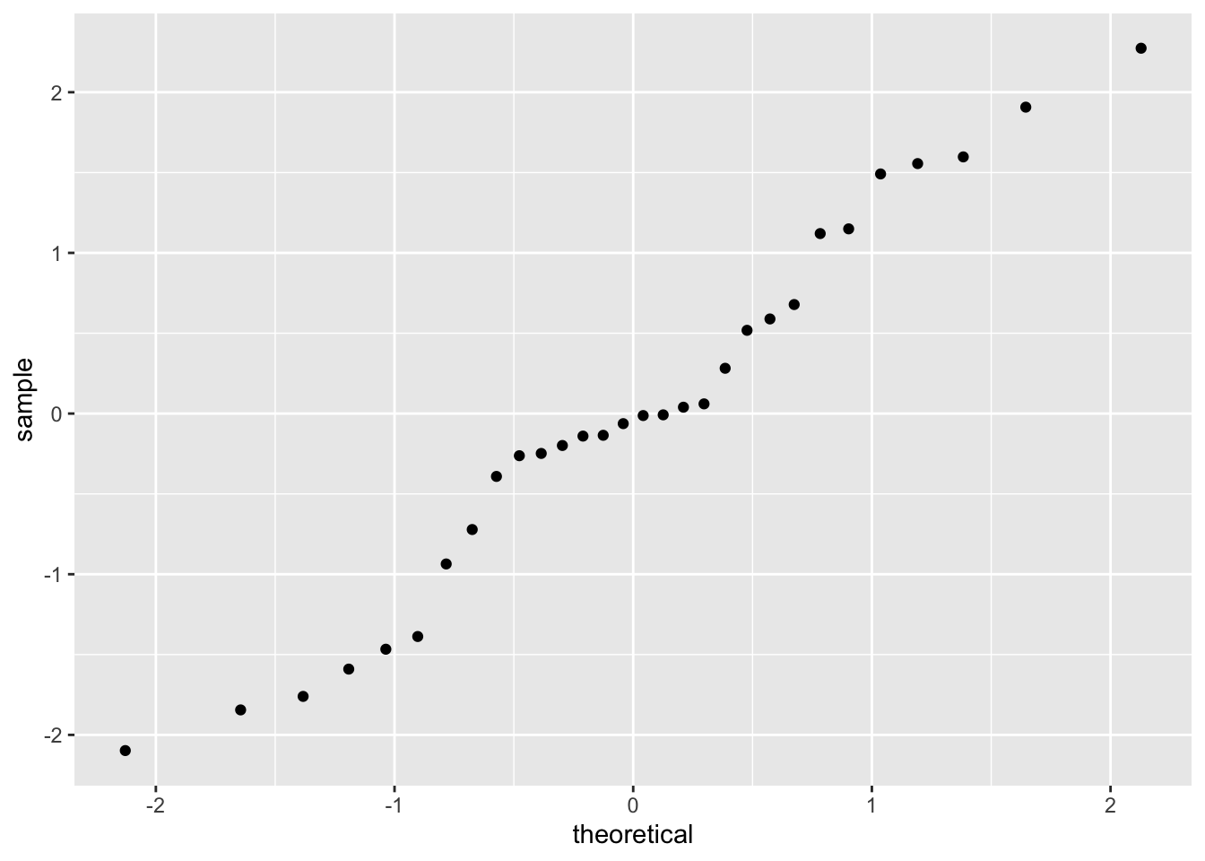
Those look a bit wonky. When residuals are not normal, the assumption that the data are random doesn’t hold, so that’s a big issue. You might need to revisit your sampling strategy or your model: are predictors missing? You can read more in Pek, Wong, and Wong (2018).

Next, our slope residuals:

l2_data %>% 
  ggplot(mapping = aes(x = slope_resid)) +
  geom_histogram(binwidth = .50)

l2_data %>% 
  ggplot(mapping = aes(sample = slope_resid)) +
  stat_qq()

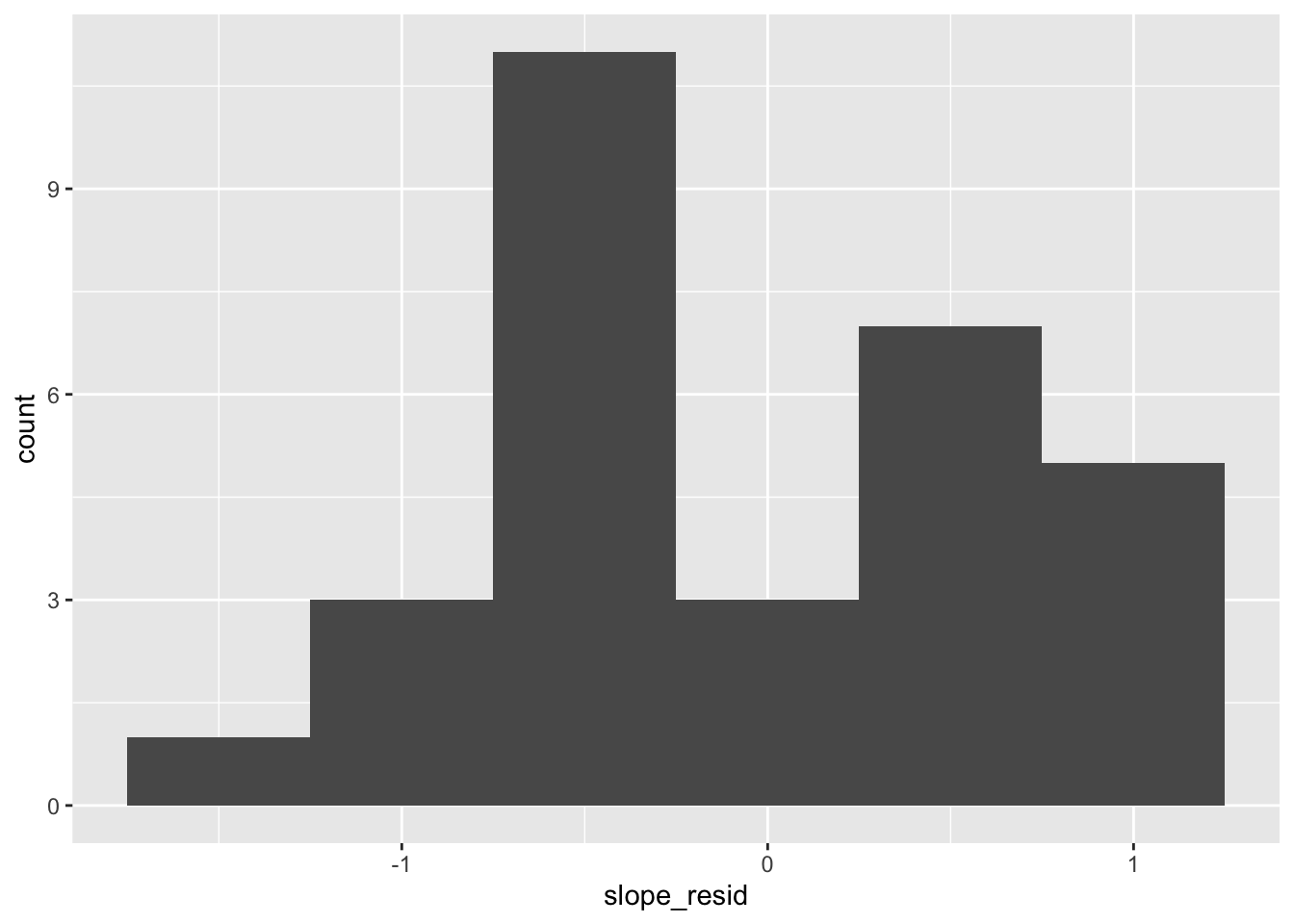
Similar issue: wonky and potentially concerning.

12.2.8 Assumption 5: Residuals at Level-1 and Level-2 are Independent

Our residuals at level-1 and level-2 should not be related to each other. We can check that with scatterplots and calculating correlations. To do so, we first need to add our level-2 residuals to our level-1 dataset. As mentioned, each school only has one level-2 intercept residual and one level-2 slope residual, but as many level-1 residuals as there are students in that school To add our level-2 residuals to the dataset, then, we need to replicate them X times, where X is the number of students in a school. For example, if a school has 10 students, we need to repeat the level-2 residuals 10 times. (This is how level-2 predictors are encoded, too: for a school with 10 students, the mean values of SES for that school repeats 10 times in the dataset.)

To do that, let’s use the replication function rep with the times argument to repeat each value X times. We can find the number of students per school as follows:

n_per_school <- data %>% 
    group_by(SCHOOL) %>% # group by school
    select(SCHOOL) %>% # we just want to count schools
    count() %>% 
    ungroup() %>% 
    select(n) %>% 
    unlist()

Then let’s create vectors of level-1 and level-2 residuals that repeat X times:

data$intercept_resid <- rep(l2_data$intercept_resid, times = n_per_school)
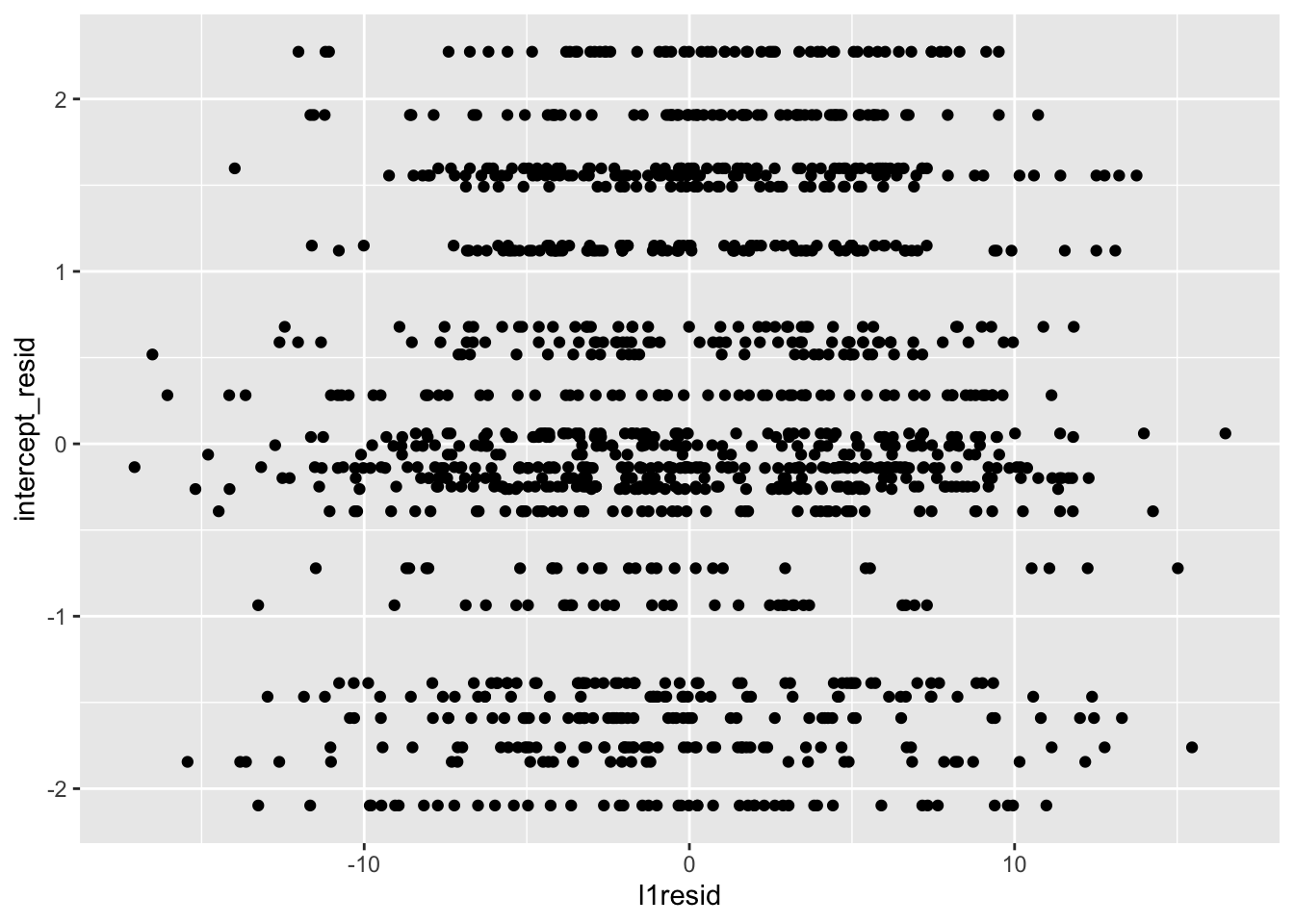
data$slope_resid <- rep(l2_data$slope_resid, times = n_per_school)

Now that we have a dataset with all of our residuals, let’s assess whether the level-1 and level-2 residuals are correlated with our trusty scatterplots and correlations. First, level-2 intercept residuals and level-1 residuals.

data %>% 
  ggplot(mapping = aes(x = l1resid, y = intercept_resid)) +
  geom_point()

cor.test(data$l1resid, data$intercept_resid)

## 
##  Pearson's product-moment correlation
## 
## data:  data$l1resid and data$intercept_resid
## t = 2.7251, df = 1327, p-value = 0.006512
## alternative hypothesis: true correlation is not equal to 0
## 95 percent confidence interval:
##  0.02091225 0.12785972
## sample estimates:
##        cor 
## 0.07460049

This looks odd at first, but the striation is because for any one level-2 residual there are multiple level-1 residuals. This looks decent; for each level-2 residual, there seems to be a decent spread of level-1 residuals. We would be concerned if level-1 residuals were clustering so that, say, for lower level-2 residuals there were also lower level-1 residuals or vice versa. Our correlation is also quite small, emphasizing that things seem fine.

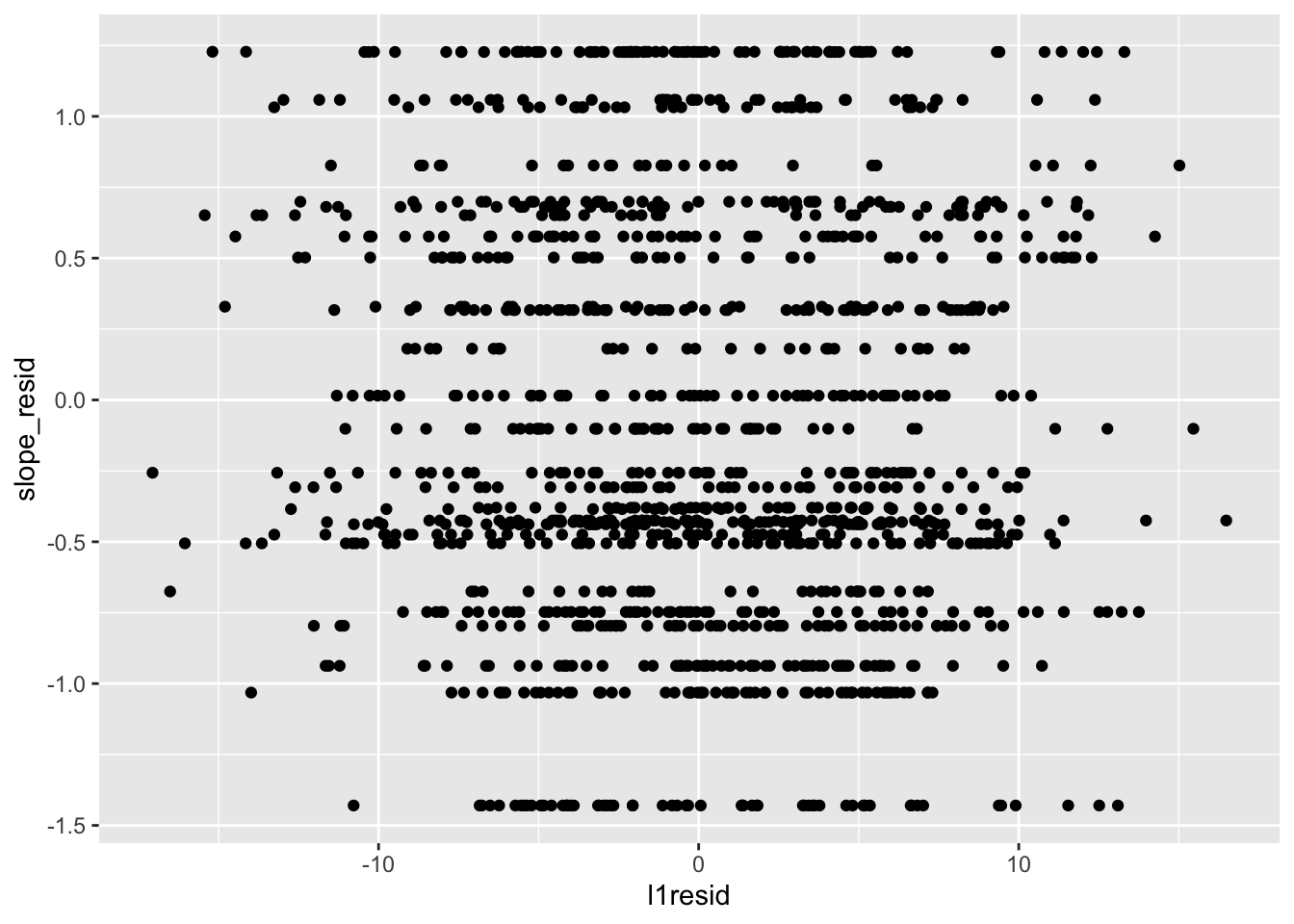
Next, level-1 residuals with level-2 slope residuals:

data %>% 
  ggplot(mapping = aes(x = l1resid, y = slope_resid)) +
  geom_point()

cor.test(data$l1resid, data$slope_resid)

## 
##  Pearson's product-moment correlation
## 
## data:  data$l1resid and data$slope_resid
## t = -1.666, df = 1327, p-value = 0.09595
## alternative hypothesis: true correlation is not equal to 0
## 95 percent confidence interval:
##  -0.099214249  0.008106189
## sample estimates:
##         cor 
## -0.04568585

This similarly looks fine.

12.2.9 Assumption 6: Level-1 Residuals Independent of Level-2 Predictors, Level-2 Residuals Independent of Level-1 Predictors

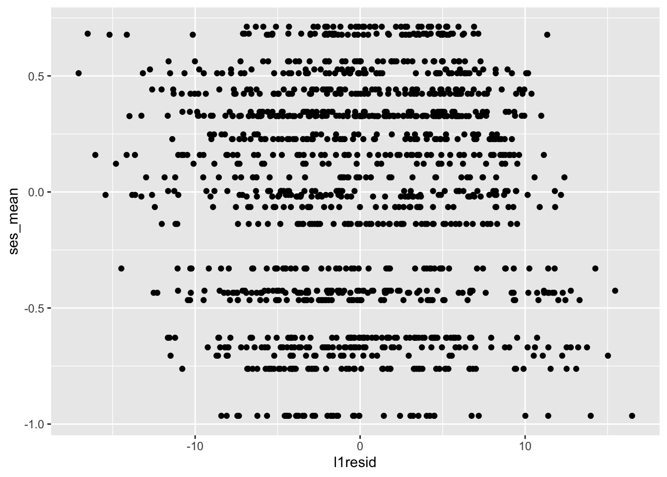
We’ve tested that our residuals are independent of predictors at their same level — level-1 residuals with ses_cwc and level-2 residuals with ses_mean. We also want residuals to be independent of predictors at the other level — level-1 residuals independent of ses_mean and level-2 residuals independent of ses_cwc. How do we test this? Scatterplots and correlations, of course. Let’s check level-1 residuals first:

data %>% 
  ggplot(mapping = aes(x = l1resid, y = ses_mean)) +
  geom_point()

cor.test(data$l1resid, data$ses_mean)

## 
##  Pearson's product-moment correlation
## 
## data:  data$l1resid and data$ses_mean
## t = -0.000000000000042298, df = 1327, p-value = 1
## alternative hypothesis: true correlation is not equal to 0
## 95 percent confidence interval:
##  -0.05377213  0.05377213
## sample estimates:
##                      cor 
## -0.000000000000001161143

The scatterplot looks like there might be a pattern where lower values on ses_mean are associated with higher residuals, but the correlation belies this.

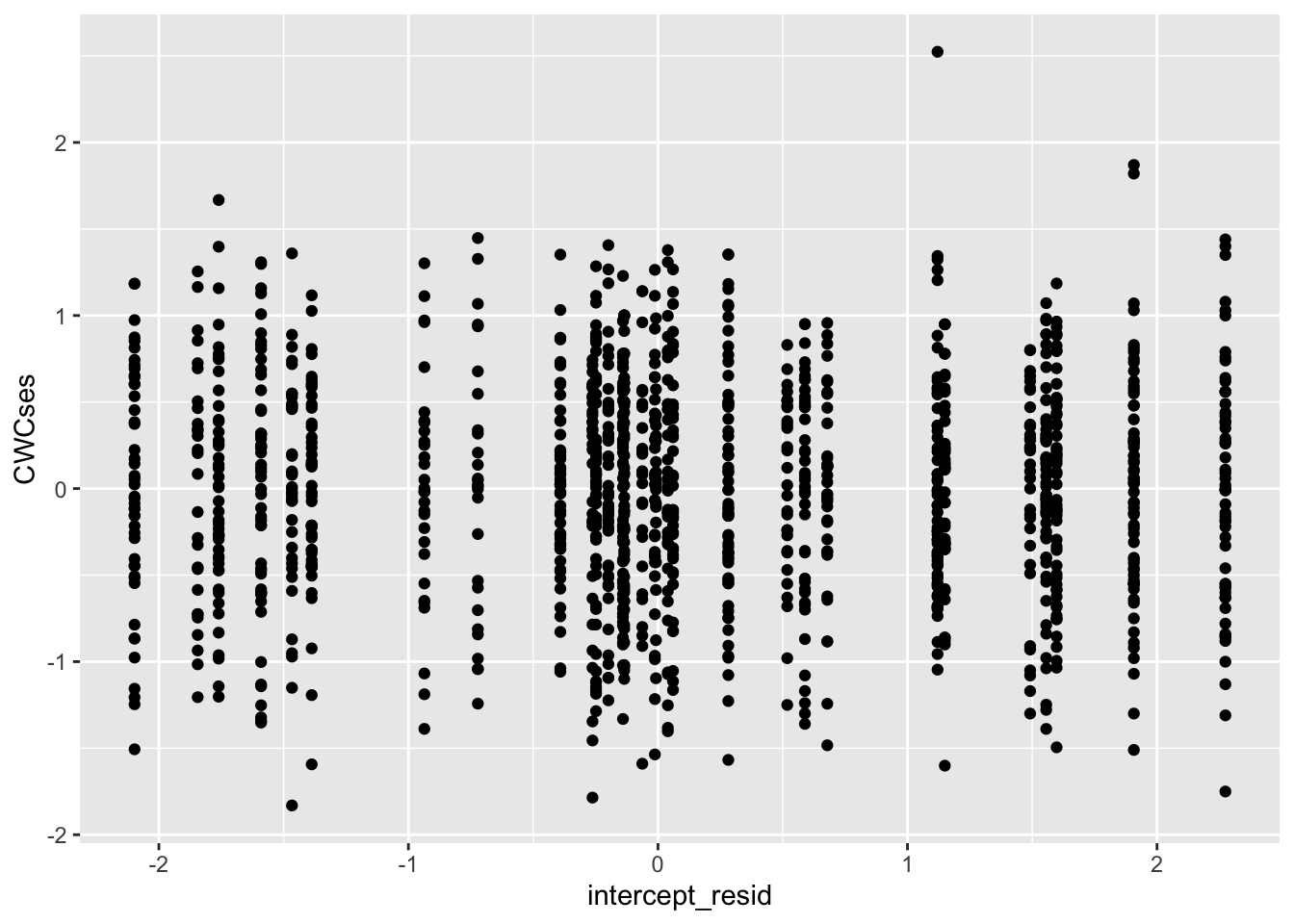
Next level-2 intercept residuals:

data %>% 
  ggplot(mapping = aes(x = intercept_resid, y = CWCses)) +
  geom_point()

cor.test(data$intercept_resid, data$CWCses)

## 
##  Pearson's product-moment correlation
## 
## data:  data$intercept_resid and data$CWCses
## t = -0.0000000000000027815, df = 1327, p-value = 1
## alternative hypothesis: true correlation is not equal to 0
## 95 percent confidence interval:
##  -0.05377213  0.05377213
## sample estimates:
##                        cor 
## -0.00000000000000007635609

Looks good!

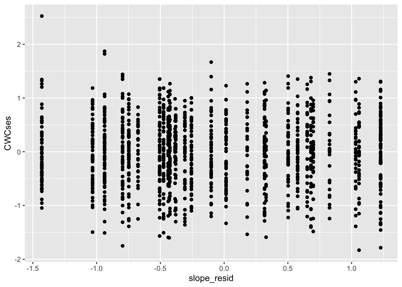
And finally level-2 slope residuals:

data %>% 
  ggplot(mapping = aes(x = slope_resid, y = CWCses)) +
  geom_point()

cor.test(data$slope_resid, data$CWCses)

## 
##  Pearson's product-moment correlation
## 
## data:  data$slope_resid and data$CWCses
## t = -0.0000000000000019141, df = 1327, p-value = 1
## alternative hypothesis: true correlation is not equal to 0
## 95 percent confidence interval:
##  -0.05377213  0.05377213
## sample estimates:
##                        cor 
## -0.00000000000000005254428

Looks great!

12.3 Conclusion

In this chapter, we reviewed the assumptions underlying multilevel models and examined some methods to assess them.

This is the last chapter of the book! We’ve covered the fundamentals: when and why you would use a multilevel model, models of varying complexity and completeness, and considerations as you build your models like estimation, various data structures, and interpreting effect sizes. Thank you for reading. If you have any suggestions or feedback, feel free to get in touch on Twitter (Mairead, Jessica) or on GitHub.

12.4 Further Reading

Pek, J., Wong, O., & Wong, A. C. M. (2018). How to Address Non-normality: A Taxonomy of Approaches, Reviewed, and Illustrated. Frontiers in Psychology, 9. doi:10.3389/fpsyg.2018.02104

Snijders, T. A. B., & Bosker, R. J. (2011). Multilevel Analysis: An Introduction to Basic and Advanced Multilevel Modeling: SAGE Publications.

Level	Equation
Level 1	\(mathach_{ij} = \beta_{0j} + \beta_{1j}cwc\_ses + R_{ij}\)
Level 2	\(\beta_{0j} = \gamma_{00} + \gamma_{10}ses\_mean + U_{0j}\)
	\(\beta_{1j} = \gamma_{10} + \gamma_{11}ses\_mean + U_{1j}\)
Combined	\(math_{ij} = \gamma_{00} + \gamma_{01}ses\_mean + \gamma_{10}cwc\_ses + \gamma_{11}cwc\_ses*ses\_mean + U_{0j} + U_{1j}cwc\_ses + R_{ij}\)