Chapter 6 Random Effects and Cross-level Interactions
6.1 Learning Objectives
In this chapter, we will introduce cross-level interactions and random effect covariances.
The learning objectives for this chapter are:
- Code and interpret models with random slope effects and cross-level interactions;
- Interpret meaning of different elements of a Tau matrix;
- Visualize a random effect covariance using Empirical Bayes estimates.
All materials for this chapter are available for download here.
6.2 Data Demonstration
The data for this chapter were taken from chapter 3 of Heck, R. H., Thomas, S. L., & Tabata, L. N. (2011). Multilevel and Longitudinal Modeling with IBM SPSS: Taylor & Francis. Students are clustered within schools in the data.
6.2.1 Load Data and Dependencies
For this data demo, we will use the following packages:
library(dplyr) # for data manipulation
library(ggplot2) # for visualizations
library(lme4) # for multilevel models
library(lmerTest) # for p-values
And the same dataset of students’ math achievement:
6.2.2 MLM with Random Slope Effect
As a reminder, in Chapter 4 we made the following scatterplot visualizing the relationship between math achievement and socioeconomic status across different schools:
data %>%
  filter(schcode <= 10) %>%
  ggplot(mapping = aes(x = ses, y = math, colour = factor(schcode))) +
  geom_point() +
  geom_smooth(mapping = aes(group = schcode), method = "lm", se = FALSE, fullrange = TRUE) +
  labs(colour = "schcode")
## `geom_smooth()` using formula = 'y ~ x'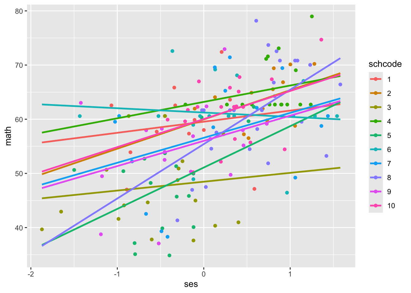
As we can see, the intercept and slope values are quite different across schools. For example, school 3 has an intercept around 38 and a small positive slope, whereas school 8 has an intercept around 55 and a larger positive slope. In Chapter 5, we modelled the relationship between math achievement and SES as follows:
| Level | Equation |
|---|---|
| Level 1 | \(math_{ij} = \beta_{0j} + \beta_{1j}ses_{ij} + R_{ij}\) |
| Level 2 | \(\beta_{0j} = \gamma_{00} + U_{0j}\) |
| \(\beta_{1j} = \gamma_{10}\) | |
| Combined | \(math_{ij} = \gamma_{00} + \gamma_{1j}ses_{ij} + U_{0j} + R_{ij}\) |
We did not assume all schools had the same mean math achievement: we modelled the variation in intercepts by adding a random intercept term (U_{0j}) to our model, which estimated the variances in intercepts across schools. However, we assumed that all schools had the same slope by only estimating the average effect of SES, and not a variance around that slope. That doesn’t seem accurate; look at our scatterplot and the variability in slopes! We can model this variance in slopes between schools by adding a random slope term to our model. The following equations describe this model:
| Level | Equation |
|---|---|
| Level 1 | \(math_{ij} = \beta_{0j} + \beta_{1j}ses_{ij} + R_{ij}\) |
| Level 2 | \(\beta_{0j} = \gamma_{00} + U_{0j}\) |
| \(\beta_{1j} = \gamma_{10} + U_{1j}\) | |
| Combined | \(math_{ij} = \gamma_{00} + \gamma_{1j}ses_{ij} + U_{0j} + U_{1j}ses_{ij} + R_{ij}\) |
With this model, we’ll now be estimating 6 parameters — 2 fixed effects, 3 random effect variances, and a random effect covariance:
- \(\gamma_{00}\): the fixed effect for the intercept, controlling for
ses; - \(\gamma_{10}\): the fixed effect for the slope of
ses; - \(\sigma^2\): a random effect variance capturing the variance of students around their school’s mean math achievement, controlling for
ses; - \(\tau_0^2\): a random effect variance for the intercept capturing the variance of schools around the intercept, controlling for
ses; - \(\tau_1^2\): a random effect variance for the slope capturing variance of school slopes around the grand mean slope, controlling for
ses; - \(\tau_{01}\): a random effect covariance capturing how the intercept variance and slope variance relate to each other.
The random effect covariance \(\tau_{01}\) quantifies the relationship between \(\tau_0^2\) and \(\tau_1^2\). It is interpreted like any other covariance, as the unstandardized relationship, but lme4 also outputs the standardized form, the correlation. If the covariance is positive, then a higher intercept value is associated with a higher slope. If negative, a higher intercept value is associated with a lower slope. If near-zero, there is minimal/no relationship between the intercept and slope values.
In our example, that would indicate schools with higher mean levels of math achievement at the intercept of ses = 0 would also have a larger slope of ses. If the covariance is negative, then a higher intercept value is associated with a lower slope. In our example, schools with higher intercepts of math achievement at ses = 0 would have lower slopes for ses. We’ll look at the actual random effect covariance in a moment.
To estimate a random slope effect in lme4, you place the predictor for which you want a random slope before the | in the code as follows:
## boundary (singular) fit: see help('isSingular')## Linear mixed model fit by REML. t-tests use Satterthwaite's method ['lmerModLmerTest']
## Formula: math ~ ses + (1 + ses | schcode)
## Data: data
##
## REML criterion at convergence: 48190.1
##
## Scaled residuals:
## Min 1Q Median 3Q Max
## -3.8578 -0.5553 0.1290 0.6437 5.7098
##
## Random effects:
## Groups Name Variance Std.Dev. Corr
## schcode (Intercept) 3.2042 1.7900
## ses 0.7794 0.8828 -1.00
## Residual 62.5855 7.9111
## Number of obs: 6871, groups: schcode, 419
##
## Fixed effects:
## Estimate Std. Error df t value Pr(>|t|)
## (Intercept) 57.6959 0.1315 378.6378 438.78 <2e-16 ***
## ses 3.9602 0.1408 1450.7730 28.12 <2e-16 ***
## ---
## Signif. codes: 0 '***' 0.001 '**' 0.01 '*' 0.05 '.' 0.1 ' ' 1
##
## Correlation of Fixed Effects:
## (Intr)
## ses -0.284
## optimizer (nloptwrap) convergence code: 0 (OK)
## boundary (singular) fit: see help('isSingular')Note that the 1 indicates a random intercept term, and is a default setting so you can also estimate both a random intercept and slope with just (ses|schcode). If you want to exclude the random intercept from the model you need to write (0 + ses|schcode) to override the default.
Let’s look at our fixed effects. Per the intercept, the average math achievement at mean SES (ses = 0) is 57.70. A one-standard-deviation increase in ses across all private schools is associated with a 3.96-point increase in math achievement.
From our random effect variances, the variance term describing how schools vary around the intercept (at mean ses) is 3.20 (\(\tau_0^2\)), the variance term describing how school SES slopes vary around the grand mean slope is 0.78 (\(\tau_1^2\)), and the variance term describing how students vary around their school’s mean math achievement is 62.59 (\(\sigma^2\)). We can find our random effect covariance by examining our Tau matrix. The Tau matrix is called a Tau matrix because it contains the estimates for our random effect variances, or Taus: \(\tau_0^2\), \(\tau_1^2\), etc. We have always been estimating a Tau matrix, but when we only had a random intercept it was just a 1-by-1 matrix of the random intercept term \(\tau_0^2\).
## 2 x 2 sparse Matrix of class "dsCMatrix"
##             (Intercept)        ses
## (Intercept)    3.204184 -1.5802590
## ses           -1.580259  0.7793617
The code looks a little busy, but there are two steps. First, we extract our random effects variance-covariance matrix (Tau matrix) with VarCorr(ses_l1_random). Then, we use the bdiag() function from the Matrix package to construct a matrix that’s easy for us to read at a glance.
In the first row and first column, we have our intercept variance term \(\tau_0^2\), 3.20. In the second row and second column, we have our slope variance term, \(\tau_1^2\), 0.78. In the second row and first column OR in the first row and second column, we have our random effect covariance, -1.58. This negative covariance indicates that for higher intercepts, the slope value is lower: the relationship between SES and math achievement decreases as mean math achievement increases. The matrix we’ve shown here only includes the level-2 random effect variances organized in matrix form, which you may see in other software programs and which can be easier to read. Information about the relationship between random effect variances is also output by lme4 under the “Random effects:” section. The lme4 output includes all random effect variances in variance and standard deviation units, as well as the correlation (not covariance) between the intercept and slope variances.
We can convert the covariance between \(\tau_0^2\) and \(\tau_1^2\) to the correlation using the standard deviations of each:
\[corr = \frac{cov(X, Y)}{sd_x*sd_y}\]
We have our covariance from our Tau matrix: -1.58. We can see the standard deviations in the lme4 output: the standard deviation of the intercept variance is 1.79, the standard deviation of the slope variance 0.88. We can then compute the correlation:
## [1] -1.003047So there is a correlation of -1 between the intercept variance and slope variance, which matches the printed output of -1.00 under the “Corr” column in the “Random effects” section of the lme4 output.
Let’s visualize the relationship using Empirical Bayes estimates (see Chapter 4 for more on EB estimates) of the intercepts and slopes for each school; we expect to see a negative relationship between them.
empirical_bayes_data <- ranef(ses_l1_random) # extract random effects for each school

empirical_bayes_intercepts <- empirical_bayes_data$schcode["(Intercept)"]

empirical_bayes_slopes <- empirical_bayes_data$schcode["ses"] # extracts the SES/slope EB estimates from the list

bind_cols(empirical_bayes_intercepts, empirical_bayes_slopes) %>%  # combine EB slopes and intercepts into a useable dataframe for graphing
  ggplot(mapping = aes(x = ses, y = `(Intercept)`)) +
  geom_point()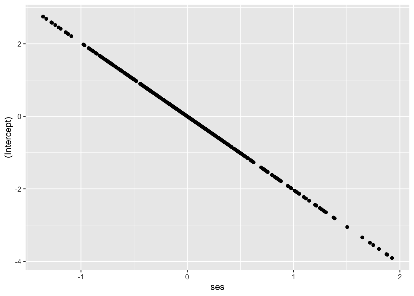
Looks like we expect! That’s a covariance of -1.58 visualized.
Finally, note that we get a convergence issue with this model: boundary (singular) fit: see help('isSingular'). For now, we’re going to ignore that. In Chapter 7 we will focus on estimation issues and troubleshooting.
6.2.3 MLM with Crosslevel Effect
In Chapter 5, we added the level-2 variable of school type (public = 0 for public schools, public = 1 for private schools) as a predictor of the intercept to answer the question: how does school type affect math achievement scores when ses = 0? Do public schools have higher or lower intercepts than private schools? The following equations described that model:
| Level | Equation |
|---|---|
| Level 1 | \(math_{ij} = \beta_{0j} + \beta_{1j}ses_{ij} + R_{ij}\) |
| Level 2 | \(\beta_{0j} = \gamma_{00} + \gamma_{10}public_j + U_{0j}\) |
| \(\beta_{1j} = \gamma_{10}\) | |
| Combined | \(math_{ij} = \gamma_{00} + \gamma_{01}public_{j} + \gamma_{10}ses_{ij} + U_{0j} + R_{ij}\) |
What if we want to know how school type affects the slope of ses, though? In other words, is there a difference in the effect of SES on math achievement in a private or public school? We can answer this question by adding school type as a predictor of SES slopes and create a cross-level interaction. This is an interaction because it allows us to estimate a different slope based on school type, whereas our previous model assumed the relationship between SES and math achievement was the same for both school types. The logic is the same as in regular regression.
We can describe this model with the following equations. Note that we are also including our slope random effect variance (\(\tau_1^2\) / \(U_{1j}\)), which allows the slopes to vary across schools. This is logically consistent with the idea that slopes might vary due to school type, but not required. We could run this model without random slopes.
| Level | Equation |
|---|---|
| Level 1 | \(math_{ij} = \beta_{0j} + \beta_{1j}ses_{ij} + R_{ij}\) |
| Level 2 | \(\beta_{0j} = \gamma_{00} + \gamma_{10}public_j + U_{0j}\) |
| \(\beta_{1j} = \gamma_{10} + \gamma_{11}public_j + U_{1j}\) | |
| Combined | \(math_{ij} = \gamma_{00} + \gamma_{01}public_{j} + \gamma_{10}ses_{ij} + \gamma_{11}ses_{ij}*public_j + U_{0j} + U_{1j}public_{j} + R_{ij}\) |
With this model, we will be estimating 8 parameters — 4 fixed effects, 3 random effect variances, and a random effect covariance:
- \(\gamma_{00}\): the fixed effect for the intercept, controlling for
sesandpublic; - \(\gamma_{01}\): the fixed effect for the slope of
public, controlling forses; - \(\gamma_{10}\): the fixed effect for the slope of
ses, controlling forpublic; - \(\gamma_{11}\): the fixed effect for the effect of
publicon the slope ofses; - \(\sigma^2\): a random effect variance capturing the variance of students around their school’s mean math achievement, controlling for
sesandpublic; - \(\tau_0^2\): a random effect variance for the intercept capturing the variance of schools around the intercept, controlling for
sesandpublic; - \(\tau_1^2\): a random effect variance for the slope capturing variance of school slopes around the grand mean slope, controlling for
sesandpublic; - \(\tau_{01}\): a random effect covariance capturing how the intercept variance and slope variance relate to each other.
A cross-level interaction is interpreted like an interaction in regular regression: the effect of school type on the effect of SES on math achievement. Like in regular regression interactions, it can also be interpreted as the effect of SES on school type on math achievement. And as in regular regression, either interpretation is accurate, but one of the other might be more intuitive for a specific research question.
Let’s run our model:
crosslevel_model <- lmer(math ~ 1 + ses + public + ses:public + (1 + ses|schcode), data = data, REML = TRUE)## boundary (singular) fit: see help('isSingular')## Linear mixed model fit by REML. t-tests use Satterthwaite's method ['lmerModLmerTest']
## Formula: math ~ 1 + ses + public + ses:public + (1 + ses | schcode)
## Data: data
##
## REML criterion at convergence: 48187.1
##
## Scaled residuals:
## Min 1Q Median 3Q Max
## -3.8509 -0.5593 0.1294 0.6412 5.6998
##
## Random effects:
## Groups Name Variance Std.Dev. Corr
## schcode (Intercept) 3.2144 1.7929
## ses 0.8013 0.8951 -1.00
## Residual 62.5555 7.9092
## Number of obs: 6871, groups: schcode, 419
##
## Fixed effects:
## Estimate Std. Error df t value Pr(>|t|)
## (Intercept) 57.72440 0.25183 382.39815 229.216 <2e-16 ***
## ses 4.42383 0.27427 1283.55622 16.130 <2e-16 ***
## public -0.02632 0.29472 387.41741 -0.089 0.9289
## ses:public -0.62520 0.31957 1363.95273 -1.956 0.0506 .
## ---
## Signif. codes: 0 '***' 0.001 '**' 0.01 '*' 0.05 '.' 0.1 ' ' 1
##
## Correlation of Fixed Effects:
## (Intr) ses public
## ses -0.232
## public -0.852 0.197
## ses:public 0.198 -0.858 -0.250
## optimizer (nloptwrap) convergence code: 0 (OK)
## boundary (singular) fit: see help('isSingular')Note that we can include interactions in two ways. Here, we are using verbose code, listing the individual effects (ses and public) and indicating their interaction with ses:public. You can also capture all of this information with an asterisk: ses*public is equivalent to ses + public + ses:public.
We have a convergence warning again: boundary (singular) fit: see help('isSingular'), and again we’re going to ignore it for now (see Chapter 7 for a deeper dive into these issues).
Let’s look at our fixed effects. Per the intercept, the average math achievement across all private schools (public = 0) at mean SES (ses = 0) is 57.72. A one-standard-deviation increase in ses across all private schools is associated with a 4.42-point increase in math achievement. Public schools (public = 1) at mean ses have a -0.02-point decrease on average in math achievement relative to private schools. The effect of ses on math achievement is lower in public schools by -0.63 points on average, which quantifies the interaction. We can calculate the expected slope for SES in public schools by using these coefficients: 4.42 - 0.63 = 3.79, so a one-unit increase in SES in public schools is associated with a 3.79-unit increase in math achievement, less of an affect than at private schools.
From our random effect variances, the variance term describing how schools vary around the intercept (at mean SES at public schools) is 3.21, the variance of school slopes around the grand mean is 0.80, and the variance term describing how students vary around their school means is 62.56. We can see our random effect covariance of -1.6 with our Tau matrix, indicating that schools with higher values of mean math achievement at the intercept of ses = 0 have lower slopes of ses.
## 2 x 2 sparse Matrix of class "dsCMatrix"
##             (Intercept)        ses
## (Intercept)    3.214435 -1.6048897
## ses           -1.604890  0.8012825
Like in other chapters, you can also calculate variance reduced at level-1 and level-2 to examine the impact of adding our cross-level effect, which we leave as an exercise to the reader.
6.3 Conclusion
In this chapter, we added random slope effects at level-1 and a cross-level interaction to our model, examined the Tau matrix, and interpreted random effect covariances. In doing so, we ran into some convergence issues (that ?isSingular warning). In Chapter 7, we’ll delve into model estimation options, problems, and troubleshooting.