Chapter 8 Centering Options and Interpretations
8.1 Learning Objectives
In this chapter, we will review options for and interpretations of centering variables in multilevel models. The examples are adapted from Dr. Dan McNeish’s lecture (thanks Dan!), and you can see an overview of his other work here.
The learning objectives for this chapter are:
- Review centering options and interpretation in linear regression.
- Differentiate between total, within, between, and contextual effects.
- Understand the difference between within-cluster and grand-mean centering and when to use each strategy.
- Estimate and interpret models using both within-cluster and grand-mean centering.
All materials for this chapter are available for download here.
8.2 Data Demonstration
The data for this chapter were taken from chapter 3 of Heck, R. H., Thomas, S. L., & Tabata, L. N. (2011). Multilevel and Longitudinal Modeling with IBM SPSS: Taylor & Francis. Students are clustered within schools in the data.
8.2.1 Load Data and Dependencies
For this data demo, we will use the following packages:
library(dplyr) # for data manipulation
library(magrittr) # for assignment pipe %<>%
library(lme4) # for multilevel models
library(lmerTest) # for p-values
And the same dataset of students’ math achievement:
8.2.2 Why Center Variables?
If you’ve worked with single-level regression before, you’re probably already familiar with centering variables. Centering in regression facilitates interpretation of the intercept, which is the average value of your outcome variable when all predictors are set to zero. If your predictors do not have meaningful zero points, then the intercept can be non-sensical. For example, imagine we were predicting the number of goals scored by players in an adult hockey league based on their age in a simple regression:
\(goals_{i} = \beta_{0} + \beta_{1}age_{i} + \epsilon_{i}\)
If we had age in years without centering it, the intercept would represent the average number of goals scored by players 0 years old. There are no players in adult hockey leagues that are zero years old, so this intercept is not really useful to us. If we instead centered age, the intercept would represent the average number of goals scored by players at the average league age (maybe something like 38 years old). This is a more meaningful interpretation that lies within the range of our data.
Centering in multilevel models is also used to make coefficients more meaningful, but also changes the interpretation of coefficients and can be used to decompose total effects into estimates of the within, between, and contextual effects of a variable. Let’s dig more into those different effects.
8.2.3 Within, Between, and Contextual Effects
To define within, between, and contextual effects, let’s think about Marsh’s Big Fish-Little Pond effect. This effect describes the situation in which high achieving students in a school that is low achieving on average, will feel better about their abilities than high achieving students in a school with higher average achievement. You may have experienced this feeling when you went from being one of the best undergraduates at your institution (i.e., you were the big fish in the little pond) to feeling less confident in your abilities when you went to graduate school (i.e., when you became a small or medium sized fish in a big pond). In the example data we have students in different schools and have measured their levels of academic achievement (their grades, for example) and academic self-concept (do they feel like they’re succeeding in school?).
The within effect describes the relationship between students’ grades and their feelings of succeeding in school within a given school: how does a student’s grades affect their feelings of success? We might expect that higher grades are associated with stronger feelings of “yes, I am succeeding.”
The between effect describes the relationship between a school’s average grades and the average of students’ feelings of success: how does a school’s average grade affect students’ average feelings of success? We might expect that in higher-performing schools, the students actually feel less successful on average.
The contextual effect describes the difference in feelings of success for students with the same grades in schools with different average grades. What would happen if we plopped the same student into a different context (i.e., cluster)? We might expect that Student A with a grade of 80% in a school with an average grade of 60% feels great about their success, but what if we take that student with a grade of 80% and put them into a school with an average grade of 99%? They probably don’t feel as successful. This is the Big Fish-Little Pond effect, and it is a contextual effect: what effect does context have on the outcome variable?
We can see this illustrated in the following graph adapted from Dan McNeish’s slides:
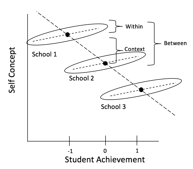
Note how the effects relate to one another: \(between\ effect = within\ effect + contextual\ effect\). One way of thinking of this is that the between effect shows the overall, average relationship, but using MLMs, we can decompose it into a within and contextual effect. To estimate these effects, We use different centering options!
8.2.4 Options for Centering in MLMs
Let’s return to our example of SES predicting math achievement to understand if there is a contextual effect of students’ achievement from being in higher or lower on average SES schools. So far, we’ve been using the following model:
| Level | Equation |
|---|---|
| Level 1 | \(math_{ij} = \beta_{0j} + \beta_{1j}ses_{ij} + R_{ij}\) |
| Level 2 | \(\beta_{0j} = \gamma_{00} + U_{0j}\) |
| \(\beta_{1j} = \gamma_{10}\) | |
| Combined | \(math_{ij} = \gamma_{00} + \gamma_{10}ses_{ij} + U_{0j} + R_{ij}\) |
## Linear mixed model fit by REML. t-tests use Satterthwaite's method ['lmerModLmerTest']
## Formula: math ~ 1 + ses + (1 | schcode)
##    Data: data
##
## REML criterion at convergence: 48215.4
##
## Scaled residuals:
##     Min      1Q  Median      3Q     Max
## -3.7733 -0.5540  0.1303  0.6469  5.6908
##
## Random effects:
##  Groups   Name        Variance Std.Dev.
##  schcode  (Intercept)  3.469   1.863
##  Residual             62.807   7.925
## Number of obs: 6871, groups:  schcode, 419
##
## Fixed effects:
##              Estimate Std. Error        df t value Pr(>|t|)
## (Intercept)   57.5960     0.1329  375.6989  433.36   <2e-16 ***
## ses            3.8739     0.1366 3914.6382   28.35   <2e-16 ***
## ---
## Signif. codes:  0 '***' 0.001 '**' 0.01 '*' 0.05 '.' 0.1 ' ' 1
##
## Correlation of Fixed Effects:
##     (Intr)
## ses -0.025
We’ve been using the variable ses which is Z-scored so 0 is equal to the mean across all students. This is a type of centering that also standardizes the units in our model. From this model, we’ve seen in previous chapters that SES has a 3.87-unit effect on achievement, meaning that math achievement is expected to increase by 3.87 units as SES increases by 1 standard deviation. This estimate cannot tell us about the effect within a school, or the contextual effect, it is an uninterpretable blend of both. We will walk through how to tease these different effects out using centering.
If we want to get our within, between, and contextual effects, we have two options (Enders and Tofighi, 2007):
- Centering within cluster (CWC)
- Centering around grand mean (CGM).
8.2.4.1 Centering Within Cluster (CWC)
Centering a variable within a cluster means each cluster will have a mean of zero. So, each school will have a mean of zero, and students’ scores on ses_cwc will reflect their variance around their school mean, not the grand mean of the whole dataset.
To center SES within cluster, we first group our dataset by school and calculate the mean SES for each cluster:
data %<>% # this symbol is an assignment operator and pipe, equivalent to data <- data %>%
  group_by(schcode) %>%
  mutate(ses_mean = mean(ses))
Then, we subtract this cluster mean from every individual student’s SES value: \(ses_{cwc} = ses - ses_{mean}\). For the students at the mean, the resulting value will be 0. Students above the mean will have positive values, and students below the mean will have negative values.
The values of ses_cwc are distributed around the mean for the cluster. The mean of the centered values for each school is now (essentially) zero:
## # A tibble: 419 × 2
##    schcode `mean(ses_cwc)`
##      <int>           <dbl>
##  1       1        6.48e-17
##  2       2       -2.56e-17
##  3       3        4.93e-17
##  4       4        6.20e-17
##  5       5       -1.31e-17
##  6       6       -1.39e-17
##  7       7        2.78e-17
##  8       8        8.54e-18
##  9       9       -1.31e-17
## 10      10       -1.11e-17
## # ℹ 409 more rows
If we estimate a model with just ses_cwc, it would look like this:
| Level | Equation |
|---|---|
| Level 1 | \(math_{ij} = \beta_{0j} + \beta_{1j}ses\_cwc_{ij} + R_{ij}\) |
| Level 2 | \(\beta_{0j} = \gamma_{00} + U_{0j}\) |
| \(\beta_{1j} = \gamma_{10}\) | |
| Combined | \(math_{ij} = \gamma_{00} + \gamma_{10}ses\_cwc_{ij} + U_{0j} + R_{ij}\) |
Here, \(\gamma_{10}\) represents how students vary around their school mean, which is our within effect. It only captures the effect of SES on achievement within schools, if we run this model we get an intercept of 57.67 and an effect for ses_cwc of 3.19 indicating that on average, within a school an increase in SES to one standard deviation above the mean is associated with an increase in math achievement of 3.19.
## Linear mixed model fit by REML. t-tests use Satterthwaite's method ['lmerModLmerTest']
## Formula: math ~ 1 + ses_cwc + (1 | schcode)
##    Data: data
##
## REML criterion at convergence: 48482.5
##
## Scaled residuals:
##     Min      1Q  Median      3Q     Max
## -3.6436 -0.5628  0.1413  0.6375  5.6268
##
## Random effects:
##  Groups   Name        Variance Std.Dev.
##  schcode  (Intercept) 10.89    3.300
##  Residual             62.59    7.912
## Number of obs: 6871, groups:  schcode, 419
##
## Fixed effects:
##              Estimate Std. Error        df t value Pr(>|t|)
## (Intercept)   57.6732     0.1883  416.1017  306.33   <2e-16 ***
## ses_cwc        3.1903     0.1578 6451.7013   20.22   <2e-16 ***
## ---
## Signif. codes:  0 '***' 0.001 '**' 0.01 '*' 0.05 '.' 0.1 ' ' 1
##
## Correlation of Fixed Effects:
##         (Intr)
## ses_cwc 0.000
This model is incomplete. If we want our between effect (i.e., how the school averages differ from each other), we can add the aggregate back in at level 2, which is the value we calculated for each school’s mean, ses_mean:
| Level | Equation |
|---|---|
| Level 1 | \(math_{ij} = \beta_{0j} + \beta_{1j}ses\_cwc_{ij} + R_{ij}\) |
| Level 2 | \(\beta_{0j} = \gamma_{00} + \gamma_{01}ses\_mean_j + U_{0j}\) |
| \(\beta_{1j} = \gamma_{10}\) | |
| Combined | \(math_{ij} = \gamma_{00} + \gamma_{01}ses\_mean_j + \gamma_{10}ses\_cwc_{ij} + U_{0j} + R_{ij}\) |
With this model, we are estimating 5 parameters:
- \(\gamma_{00}\): the fixed effect for the intercept, controlling for
ses_cwcandses_mean(i.e., a student with school-average SES at the average school); - \(\gamma_{01}\): the fixed effect for
ses_meancontrolling forses_cwc. This is our between effect, indicating the effect of a school’s average SES on a student’s math achievement; - \(\gamma_{10}\): the fixed effect for the slope of
ses_cwccontrolling forses_mean. This is our within effect, indicating the effect of a student’s SES compared to the school average (at the average school,ses_mean= 0); - \(\tau_0^2\): a random effect variance for the intercept capturing the variance of schools around the intercept, controlling for
ses_cwcandses_mean; - \(\sigma^2\): a random effect variance capturing the variance of students around their school mean math achievement, controlling for
ses_cwcandses_mean.
Let’s estimate it:
model_cwc_l2 <- lmer(math ~ 1 + ses_cwc + ses_mean + (1|schcode), data = data, REML = TRUE)
summary(model_cwc_l2)
## Linear mixed model fit by REML. t-tests use Satterthwaite's method ['lmerModLmerTest']
## Formula: math ~ 1 + ses_cwc + ses_mean + (1 | schcode)
## Data: data
##
## REML criterion at convergence: 48137.9
##
## Scaled residuals:
## Min 1Q Median 3Q Max
## -3.7545 -0.5575 0.1312 0.6619 5.7512
##
## Random effects:
## Groups Name Variance Std.Dev.
## schcode (Intercept) 2.511 1.585
## Residual 62.628 7.914
## Number of obs: 6871, groups: schcode, 419
##
## Fixed effects:
## Estimate Std. Error df t value Pr(>|t|)
## (Intercept) 57.5467 0.1239 401.3223 464.54 <2e-16 ***
## ses_cwc 3.1903 0.1578 6448.7759 20.22 <2e-16 ***
## ses_mean 5.8920 0.2529 385.3371 23.30 <2e-16 ***
## ---
## Signif. codes: 0 '***' 0.001 '**' 0.01 '*' 0.05 '.' 0.1 ' ' 1
##
## Correlation of Fixed Effects:
## (Intr) ss_cwc
## ses_cwc 0.000
## ses_mean -0.052 0.000The average student math achievement at the average school is 57.55. A one-unit increase in SES within a school is associated with a 3.19-unit increase in math achievement. A one-unit increase in the school’s average SES is associated with a 5.89-unit increase in math achievement.
Recall our earlier formula detailing the relationship between the within, between, and contextual effects: \(between\ effect = within\ effect + contextual\ effect\). Armed with our between effect (\(\gamma_{01}\)) and within effect (\(\gamma_{10}\)), we can reorganize this equation and calculate our contextual effect: \(contextual = between - within = \gamma_{01} - \gamma_{10} = 5.89 - 3.19 = 2.70\), so with two hypothetical students with the same level of SES, the one in the school with higher average SES has 2.70-unit higher math achievement. This represents the contextual effect of a school’s SES on math achievement.
8.2.4.2 Centering Grand Mean (CGM)
When we center a variable at the grand mean, we have information about how individuals vary around the mean of all individuals. So students’ scores on ses_cgm will reflect their variance around the mean of all students.
To center SES at the grand mean, we first calculate the grand mean:
data %<>%
  ungroup() %>% # remove the grouping by school that we added in the CWC section
  mutate(ses_grand_mean = mean(ses))
Then, we subtract this grand mean from every individual student’s SES value: \(ses_{cgm} = ses - ses\_grand\_mean\). For the students at the grand mean, the resulting value will be 0. Students above the mean will have positive values, and students below the mean will have negative values.
The values of ses_cgm are distributed around the grand mean. The mean of the students’ values of ses_cgm is now (essentially) zero.
## # A tibble: 1 × 1
##   `mean(ses_cgm)`
##             <dbl>
## 1        4.73e-17
If we estimate a model with just ses_cgm, it would look like this:
| Level | Equation |
|---|---|
| Level 1 | \(math_{ij} = \beta_{0j} + \beta_{1j}ses\_cgm_{ij} + R_{ij}\) |
| Level 2 | \(\beta_{0j} = \gamma_{00} + U_{0j}\) |
| \(\beta_{1j} = \gamma_{10}\) | |
| Combined | \(math_{ij} = \gamma_{00} + \gamma_{10}ses\_cgm_{ij} + U_{0j} + R_{ij}\) |
Here, \(\gamma_{10}\) represents how students vary around the grand mean. If we don’t factor out school means, then this value is an uninterpretable blend of within- and between-effects, sometimes referred to as the total effect. When we center at the grand mean, we must add the cluster mean back into into the model. (This is in contrast to centering within cluster, when we can just estimate the within effect, but to get the between effect we must add the cluster mean back into the model).
| Level | Equation |
|---|---|
| Level 1 | \(math_{ij} = \beta_{0j} + \beta_{1j}ses\_cgm_{ij} + R_{ij}\) |
| Level 2 | \(\beta_{0j} = \gamma_{00} + \gamma_{01}ses\_mean_j + U_{0j}\) |
| \(\beta_{1j} = \gamma_{10}\) | |
| Combined | \(math_{ij} = \gamma_{00} + \gamma_{01}ses\_mean_j + \gamma_{10}ses\_cgm_{ij} + U_{0j} + R_{ij}\) |
With this model, we are estimating 5 parameters:
- \(\gamma_{00}\): the fixed effect for the intercept, controlling for
ses_cgmandses_mean(i.e., a student with school-average SES at the average school); - \(\gamma_{01}\): the fixed effect for
ses_meancontrolling forses_cgm. This is our contextual effect, indicating the effect of school average SES on student math achievement at the same level of student SES; - \(\gamma_{10}\): the fixed effect for the slope of
ses_cgmcontrolling forses_mean. This is our within effect, indicating the effect of a student’s SES compared to the school average (at the average school,ses_mean= 0); - \(\tau_0^2\): a random effect variance for the intercept capturing the variance of schools around the intercept, controlling for
ses_cgmandses_mean; - \(\sigma^2\): a random effect variance capturing the variance of students around their school mean math achievement, controlling for
ses_cgmandses_mean.
Let’s estimate it in R:
cgm_model <- lmer(math ~ 1 + ses_cgm + ses_mean + (1|schcode), data = data, REML = TRUE)
summary(cgm_model)
## Linear mixed model fit by REML. t-tests use Satterthwaite's method ['lmerModLmerTest']
## Formula: math ~ 1 + ses_cgm + ses_mean + (1 | schcode)
## Data: data
##
## REML criterion at convergence: 48137.9
##
## Scaled residuals:
## Min 1Q Median 3Q Max
## -3.7545 -0.5575 0.1312 0.6619 5.7512
##
## Random effects:
## Groups Name Variance Std.Dev.
## schcode (Intercept) 2.511 1.585
## Residual 62.628 7.914
## Number of obs: 6871, groups: schcode, 419
##
## Fixed effects:
## Estimate Std. Error df t value Pr(>|t|)
## (Intercept) 57.6485 0.1240 402.6508 464.982 <2e-16 ***
## ses_cgm 3.1903 0.1578 6448.7759 20.217 <2e-16 ***
## ses_mean 2.7017 0.2981 738.7254 9.065 <2e-16 ***
## ---
## Signif. codes: 0 '***' 0.001 '**' 0.01 '*' 0.05 '.' 0.1 ' ' 1
##
## Correlation of Fixed Effects:
## (Intr) ss_cgm
## ses_cgm 0.041
## ses_mean -0.066 -0.529The average student math achievement at the average school is 57.65. For two hypothetical students with the same level of SES, the one in the school with higher average SES has 2.70-unit higher math achievement. Within a school, a one-unit increase in SES relative to the grand mean is associated with a 3.19-unit increase in math achievement.
Recall our earlier formula detailing the relationship between the within, between, and contextual effects: \(between\ effect = within\ effect + contextual\ effect\). Armed with our contextual effect (\(\gamma_{01}\)) and within effect (\(\gamma_{10}\)), we can calculate our between effect: \(between = within + contextual = \gamma_{10} + \gamma_{01} = 3.19 + 2.70 = 5.89\), so an increase in a school’s average SES by one unit is associated with an increase of 5.89-unit math achievement.
8.2.5 What Kind of Centering Should You Use?
Here is a reference table to keep track of what coefficients represent what effects in CWC or CGM models:
| Centering Option | Contextual Parameter | Within Parameter | Between Parameter |
|---|---|---|---|
| Centering Grand Mean (CGM) | \(\gamma_{01}\) | \(\gamma_{10}\) | \(\gamma_{01} + \gamma_{10}\) |
| Centering Within Cluster (CWC) | \(\gamma_{01} - \gamma_{10}\) | \(\gamma_{10}\) | \(\gamma_{01}\) |
Let’s look at our example results this way:
| Centering Option | Contextual Parameter | Within Parameter | Between Parameter |
|---|---|---|---|
| Centering Grand Mean (CGM) | 2.70 | 3.19 | 5.89 |
| Centering Within Cluster (CWC) | 2.70 | 5.89 | 3.19 |
If you’re not interested in contextual results, you can use the following shorthand for deciding whether to center around the grand mean or within cluster: if you’re interested in level-1 predictors, CWC is best because it gives an unbiased estimate of the within cluster effect and produces better estimates of the slope variance, though as we saw you can get an unbiased estimate of the within cluster effect with CGM if you add the aggregate back in at level 2. If you’re interested in level-2 predictors, but you have covariates at level-1 you want to control for, CGM is best because it controls for level-1 predictors by producing adjusted means. If you are interested in interactions (at level-1 or cross-level), use CWC to get an unbiased estimate of the within cluster slope and slope variance. See Enders & Tofighi (2007) for a detailed discussion.
8.3 Conclusion
In this chapter, we reviewed two options for centering variables in MLMs (centering within cluster and centering grand mean), when to use each option, and how to interpret coefficients under each option. In the first 8 chapters, we’ve covered a lot of the basics of MLMs. In Chapter 9, we’ll revisit a number of concepts we’ve already seen, but in the context of repeated-measure rather than the cross-sectional data we’ve been using to this point.
8.4 Further Reading
Enders, C. K., & Tofighi, D. (2007). Centering predictor variables in cross-sectional multilevel models: A new look at an old issue. Psychological Methods, 12(2), 121–138. https://doi.org/10.1037/1082-989X.12.2.121