Chapter 4 Our First Multilevel Models
4.1 Learning Objectives
In this chapter, we will run our first multilevel model to account for the clustered nature of our data and begin visualizing and understanding the variance in our data.
The learning objectives for this chapter are:
- Visualize clustering in data structures;
- Recognize when to use a multilevel model over cluster-robust standard errors;
- Explain the difference between fixed and random effects in MLMs;
- Code and interpret the null model;
- Determine how variance is distributed in a dataset.
All materials for this chapter are available for download here.
4.2 Data Demonstration
The data for this chapter were taken from chapter 3 of Heck, R. H., Thomas, S. L., & Tabata, L. N. (2011). Multilevel and Longitudinal Modeling with IBM SPSS: Taylor & Francis. Students are clustered within schools in the dataset.
4.2.1 Load Data and Dependencies
For this data demo, we will use the following packages:
library(dplyr) # for data manipulation
library(ggplot2) # for visualizations
library(lme4) # for multilevel models
library(lmerTest) # for p-values
library(performance) # for intraclass correlation
And the same dataset of students’ math achievement from chapters 2 and 3:
4.2.2 Why Multilevel Models?
In chapter 3 we talked about cluster-robust standard errors, which handle clustering as a nuisance, but doesn’t investigate it as interesting or enable multilevel research questions. But if you’re interested in the clustered structure of the data, and you want to know how clusters differ or ask questions at multiple levels, you’ll need a multilevel model. To get a sense of how the outcome is clustered, let’s start by making some graphs. Our data set contains students clustered into 419 schools. For demonstration, we will take a subset of 10 schools.
In chapter 2, we created a scatterplot with math achievement (math) on the y-axis and socioeconomic status (ses) on the x-axis. Let’s re-create that graph and overlay a line of best fit, first ignoring the clustering.
data_sub %>%
  ggplot(mapping = aes(x = ses, y = math)) +
  geom_point() +
  geom_smooth(method = "lm", se = FALSE, fullrange = TRUE)
## `geom_smooth()` using formula = 'y ~ x'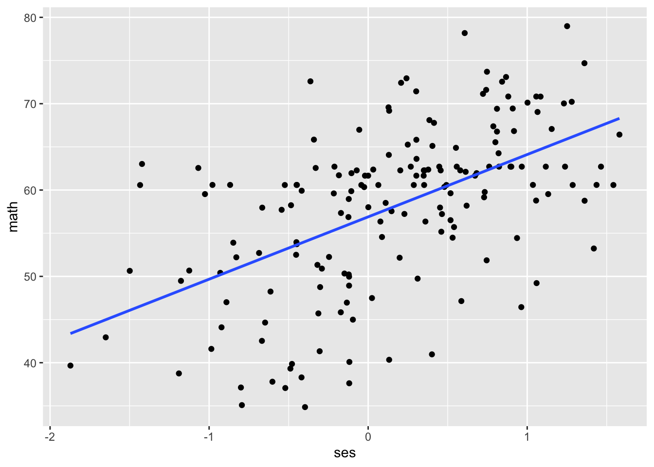
Now, let’s create the same scatterplot, this time colouring the points by school (schcode).
data_sub %>%
  ggplot(mapping = aes(x = ses, y = math, colour = factor(schcode))) +
  geom_point() +
  geom_smooth(mapping = aes(group = schcode), method = "lm", se = FALSE, fullrange = TRUE) +
  labs(colour = "schcode")
## `geom_smooth()` using formula = 'y ~ x'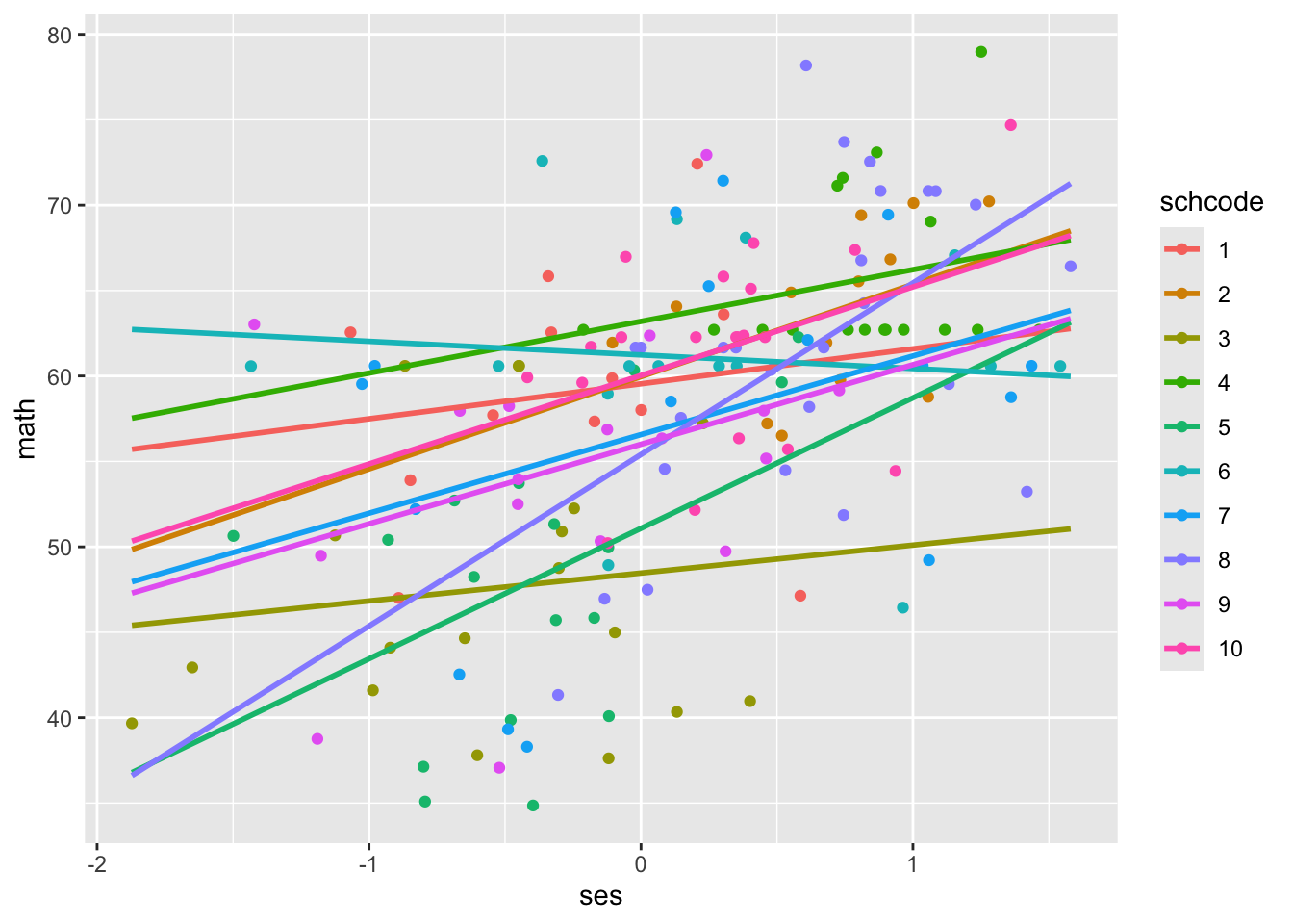
When we run a regular regression without accounting for the clustered structure of the data, we treat all schools as though they have the same intercept and slope. What do you notice about the intercepts and slopes for different schools?
The intercepts and slopes vary widely! For example, school 4 has an intercept around 62, compared to the intercept of school 3 around 49. School 8 has a relatively large positive slope, while school 6 has a slightly negative slope. With multilevel models, we can quantify this variance and ask questions about it.
4.2.3 Fixed vs Random Effects
Multilevel models have two main ingredients: fixed and random effects. For our purposes of executing and interpreting MLMs, a fixed effect is an average effect across all clusters and a random effect describes how an effect for a given cluster differs from the average. We are usually interested less in individual random effects, and more in the random effects variances that describe how effects vary across all clusters. For example, we might have a fixed effect for the intercept that describes average math achievement across all schools. Then we have a random effect variance that describes how intercepts for math achievement vary across schools. Together, the fixed effect and random effect variance describe math achievement scores across schools.
4.2.4 The Null Model
In the simplest MLM we can run, we let intercepts vary between clusters by estimating random effects for the intercepts in addition to a fixed effect. The random effect allows the intercepts to deviate from the fixed effect, the grand mean of the intercepts. As a result, this model is called the “random intercept only model,” also known as the “null model.” For our example, math achievement is our outcome variable, and the equations for the null model look like this:
| Level | Equation |
|---|---|
| Level 1 | \(math_{ij} = \beta_{0j} + R_{ij}\) |
| Level 2 | \(\beta_{0j} = \gamma_{00} + U_{0j}\) |
| Combined | \(math_{ij} = \gamma_{00} + U_{0j} + R_{ij}\) |
Let’s run the model.
## Linear mixed model fit by REML. t-tests use Satterthwaite's method ['lmerModLmerTest']
## Formula: math ~ 1 + (1 | schcode)
##    Data: data
##
## REML criterion at convergence: 48877.3
##
## Scaled residuals:
##     Min      1Q  Median      3Q     Max
## -3.6336 -0.5732  0.1921  0.6115  5.2989
##
## Random effects:
##  Groups   Name        Variance Std.Dev.
##  schcode  (Intercept) 10.64    3.262
##  Residual             66.55    8.158
## Number of obs: 6871, groups:  schcode, 419
##
## Fixed effects:
##             Estimate Std. Error       df t value Pr(>|t|)
## (Intercept)  57.6742     0.1883 416.0655   306.3   <2e-16 ***
## ---
## Signif. codes:  0 '***' 0.001 '**' 0.01 '*' 0.05 '.' 0.1 ' ' 1
In lme4, the syntax for a two-level model is lmer(DV ~ 1 + IV1 + IV2 + ... + IVp + (random_effect1 + random_effect2 + ... + random_effect3 | grouping_variable), data = dataset). Our dependent variable is math achievement (math), and we have a fixed and random effect of the intercept (represented by the 1s). Our grouping variable is school (schcode).
The key output to interpret is:
- Number of parameters
- Estimates of fixed effects
- Estimates of random effects variances
As indicated in our combined equation, we are estimating three parameters:
- \(\gamma_{00}\): the fixed effect for the intercept;
- \(\tau_0^2\): a variance for the random effects of the intercept, capturing the variance of schools around the intercept. Each \(U_{0j}\) is the residual of a school around the intercept; that is, it describes how the school’s mean math achievement at the intercept deviates from the intercept for the entire sample. Every school has a \(U_{0j}\), and the variance of all of the \(U_{0j}\)s is \(\tau_0^2\);
- \(\sigma^2\): a random effect variance capturing the variance of students around their school mean math achievement. Each student has a residual, \(R_{ij}\), and the variance of all the \(R_{ij}\)s is \(\sigma^2\).
We can double-check we’ve counted parameters correctly using the logLik function from the stats package.
## 'log Lik.' -24438.63 (df=3)The degrees of freedom listed, (df = 3), correspond to the number of parameters we’re estimating. We’ll discuss log likelihoods a bit more in chapter 7, so ignore the other number for now.
The fixed effect for the intercept is 57.67, representing the average math achievement score across all schools. The variance of schools around the intercept is 10.64, and of students around their school’s mean is 66.55.
4.2.5 Understanding Variance
4.2.5.1 Intraclass Correlation Coefficient (ICC)
The intraclass correlation coefficient quantifies the extent of clustering in a dataset. It ranges from 0 to 1 and is the quotient of the variance between clusters to the total variance: \(ICC = \frac{\tau_0^2}{\tau_0^2 + \sigma^2}\). The more extensive the impact of clustering, the more variance between clusters, the larger the ICC. The ICCs can also be interpreted as (1) the proportion of variance in the outcome that is attributable to clusters or (2) the expected correlation between the outcome from randomly selected units from a randomly selected cluster.
Per our model output, the total variance is \(\tau_0^2 + \sigma^2 = 10.64 + 66.55 = 77.19\), and the variance between schools is \(\tau_0^2\), 10.64. The ICC is then \(\frac{10.64}{77.19} = 0.138\); 13.8% of the total variance in math achievement can be attributed to school membership.
We can use the performance package to calculate this automatically:
## # Intraclass Correlation Coefficient
##
##     Adjusted ICC: 0.138
##   Unadjusted ICC: 0.138
Don’t worry about the adjusted vs conditional ICC here. In short, the adjusted ICC accounts only for the random effect variances, while the conditional ICC accounts for the fixed effect variances, too. You can read more about it here.
4.2.5.2 Plausible Values Range
Another way to understand the variance in our data is by calculating a 95% plausible values range for a given effect. For example, the intercept: given the fixed effect for the intercept (\(\gamma_{00}\)) and the variance of residuals around that fixed effect (\(\tau_0^2\)), we can describe how much the schools vary in mean math achievement by calculating a 95% plausible values range. \(95\%\ plausible\ values\ range = \gamma_{00} ± 1.96\sqrt{\tau_0^2}\).
Tau0 <- VarCorr(null_model)$schcode[1]

lower_bound <- null_model@beta - 1.96*sqrt(Tau0)
upper_bound <- null_model@beta + 1.96*sqrt(Tau0)

lower_bound
## [1] 51.28024## [1] 64.06822This range gives us a sense of the variance in school intercepts: 95% of intercepts will fall between 51 and 64. 13 points of variance is a fair amount for a scale from 0 to 100! It seems good that we’re accounting for that variance with our multilevel model, rather than treating all schools like they have the same intercept.
4.2.5.3 Empirical Bayes Estimates
As noted, every school has its own intercept residual, \(U_{0j}\). We’re not usually interested in individual residuals; rather, we’re interested in the variance of those residuals to understand the clustering in our data. But we can visualize at the individual residuals as a third way of understanding that variation. We can extract and plot the residuals as Empirical Bayes estimates, which are weighted. The random effects for the intercept (the \(U_{0j}\)s) are latent variables rather than statistical parameters, but we can estimate them to visualize how much they vary (and thus how much schools vary around the grand mean intercept). We can estimate a weighted intercept for a given group with the following equation:
\(\hat\beta_{0j}^{EB} = \lambda_j\hat\beta_{0j} + (1 - \lambda_j)\hat\gamma_{00}\)
To calculate the weighted intercept, we use the following information:
- Group mean information (\(\hat{\beta}\));
- Population mean information (\(\hat{\gamma_{00}}\));
- Weight \(\lambda_j = \frac{\tau_0^2}{\tau_0^2 + \frac{\sigma^2}{n_j}}\). The larger a cluster, the closer the denominator is to the numerator, the larger the weight.
The Empirical Bayes estimate of a residuals, \(U_{0j}\), is then the difference between the fixed effect \(\gamma_{0j}\) and the EB estimate \(\hat\beta_{0j}^{EB}\). To develop an intuition about EB estimates, let’s manually calculate the residual for the intercept for school 1, or \(U_{01}\).
First, we need the group mean math achievement, \(\hat{\beta_{01}}\):
##   mean(math)
## 1   58.99677
Next, we need the estimated population mean, \(\hat{\gamma_{00}}\). We have that from our earlier MLM: the intercept of 57.6742.
Finally, we need the weight: \(\lambda_j = \frac{\tau_0^2}{\tau_0^2 + \frac{\sigma^2}{n_j}}\). We also have \(\tau_0^2 = 10.64\) and \(\sigma^2 = 66.55\) from our earlier MLM. We need the group sample size, \(n_1\):
##    n
## 1 12
So \(\lambda_j = \frac{\tau_0^2}{\tau_0^2 + \frac{\sigma^2}{n_j}} = \frac{10.64}{10.64 + \frac{66.55}{12}} = 0.657\).
Combining this information into our Empirical Bayes formula, \(\hat\beta_{01}^{EB} = 58.545\). The residual between the intercept from our MLM — 57.6742 — and our Empirical Bayes estimate — 58.545 — is 0.87. We could repeat this manual calculation process and get an Empirical Bayes residual for every school, and then plot those residuals to visualize their distribution. Luckily, we don’t need to do this manual process 419 times; we can extract the Empirical Bayes estimates of the residuals using code:
We can double-check our manual calculation:
## # A tibble: 1 × 5
##   grpvar  term        grp   condval condsd
##   <chr>   <fct>       <fct>   <dbl>  <dbl>
## 1 schcode (Intercept) 1       0.869   1.91
Looks like the residual for school 1 (grp 1) is 0.87, just like we manually calculated! Then, we can plot the residuals to visualize their distribution.
ggplot(data = empirical_bayes_data, mapping = aes(x = condval)) + # "condval" is the name of the EB estimates returned by the ranef function above
  geom_histogram() +
  labs(x = "EB estimate of U0j")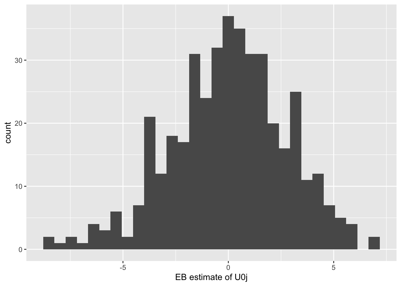
As we would expect, the residuals have a mean of 0 because the process of estimating the model is a process of minimizing the residuals. It looks like they mostly range from -5 to 5 in a normal distribution. Again, looks like our intercepts vary fairly widely between schools, so it’s a good thing we’re modelling that variation.
4.3 Conclusion
In this chapter, we discussed why and when one should use multilevel models, reviewed different ways to visualize and understand the variance in your data at different levels, and estimated our first multilevel model: the random-intercept-only model (also called the null model). In the next chapter, we’ll start adding more fixed effects.