Chapter 2 Multiple Regression Review

2.1 Learning Objectives

In this module, we will review simple and multiple linear regression to establish a strong foundation before moving onto multilevel models. Note that this is intended more as review than a comprehensive guide to regression; for the latter, we recommend https://stats.oarc.ucla.edu/other/mult-pkg/seminars/.

All materials for this chapter are available for download here.

The learning objectives for this chapter are:

Understand using file paths for project management/loading data;
Review using simple and multiple linear regression to analyze data.

2.2 Data Demonstration

In this data demo, we will first review setting up an R session, then simple and multiple linear regression.

The data for this chapter were taken from chapter 3 of Heck, R. H., Thomas, S. L., & Tabata, L. N. (2011). Multilevel and Longitudinal Modeling with IBM SPSS: Taylor & Francis. These data have a multilevel structure, which we will work with in chapter 3, but for this chapter we will ignore the clustering structure and conduct regular regression. The following variables are in this data set:

Variable	Level	Description	Values	Measurement
schcode	School	School identifier (419 schools)	Integer	Ordinal
Rid	Individual	A within-group level identifier representing a sequential identifier for each student within 419 schools.	1 to 37	Ordinal
id	Individual	Student identifier (6,871 students)	Integer	Ordinal
female	Individual	Student sex	0 = Male, 1 = Female	Scale
ses	Individual	Z-score measuring student socioeconomic status composition within the schools	-2.41 to 1.87	Scale
femses	Individual	Grand-mean-centered variable measuring student socioeconomic status by gender (female)	-2.41 to 1.85	Scale
math	Individual	Student math achievement test score	27.42 to 99.98	Scale
ses_mean	School	Grand-mean-centered variable measuring student socioeconomic status	-1.30 to 1.44	Scale
pro4yrc	School	Aggregate proportion of students who intend to study at 4-year universities	0.00 to 1.00	Scale
public	School	Dichotomous variable identifying school type	0 = Other, 1 = Public School	Scale

2.2.1 Creating R Projects

Before we get into analyzing the data, let’s start by creating a new project file for this module. R project files help you keep all of the files associated with your project – data, R scripts, and output (including figures) – in one location so you can easily navigate everything related to your project.

To create a project, open R, click “File” and “New Project…”. If you have already created a folder for this chapter, you can add an R Project to that folder by clicking “Existing Directory”; the R project file will take on the name of that folder. If you do not already have a folder, click “New Directory,” choose where you want to put your new folder and what you want to call it. The R Project file will again take on the name of your new folder.

2.2.2 Loading Data and Dependencies

Next, let’s load in the data and packages we’ll be using for this demo. We’ll be using the following packages:

library(ggplot2) # for data visualization
library(magrittr) # for pipe, %>%

You must install a given package before you can use it. For example: install.package("ggplot2"). Once you have installed a package, you can load it into any future sessions with library(package_name).

Next, let’s read in the data. If you have your code and data in the same directory, you can read the data in as follows:

data <- read.csv('heck2011.csv')

This is called a relative file path, because you’re telling your computer where to find the data relative to your current folder (a folder can also be called a “directory”). You could also use an absolute file path that fully states where your files are located, like:

read.csv('/Users/maireadshaw/open_mlm_materials/heck2011.csv')

Let’s calculate some descriptive statistics and compare them to the above table to make sure we read our data in correctly.

summary(data)

##     schcode           Rid               id           female            ses         
##  Min.   :  1.0   Min.   : 1.000   Min.   :   1   Min.   :0.0000   Min.   :-2.4140  
##  1st Qu.:103.5   1st Qu.: 5.000   1st Qu.:1718   1st Qu.:0.0000   1st Qu.:-0.5180  
##  Median :209.0   Median : 9.000   Median :3436   Median :1.0000   Median : 0.0150  
##  Mean   :209.4   Mean   : 9.196   Mean   :3436   Mean   :0.5025   Mean   : 0.0319  
##  3rd Qu.:314.5   3rd Qu.:13.000   3rd Qu.:5154   3rd Qu.:1.0000   3rd Qu.: 0.6050  
##  Max.   :419.0   Max.   :37.000   Max.   :6871   Max.   :1.0000   Max.   : 1.8730  
##      femses                math          ses_mean           pro4yrc           public      
##  Min.   :-2.4140000   Min.   :27.42   Min.   :-1.29673   Min.   :0.0000   Min.   :0.0000  
##  1st Qu.:-0.0175000   1st Qu.:52.41   1st Qu.:-0.30525   1st Qu.:1.0000   1st Qu.:0.0000  
##  Median : 0.0000000   Median :60.67   Median :-0.01050   Median :1.0000   Median :1.0000  
##  Mean   : 0.0000984   Mean   :57.73   Mean   : 0.03179   Mean   :0.8689   Mean   :0.7306  
##  3rd Qu.: 0.0000000   3rd Qu.:62.38   3rd Qu.: 0.29560   3rd Qu.:1.0000   3rd Qu.:1.0000  
##  Max.   : 1.8540000   Max.   :99.98   Max.   : 1.44315   Max.   :1.0000   Max.   :1.0000

That looks good, so let’s proceed to conducting regressions.

2.2.3 Simple Linear Regression

Let’s run a simple linear regression predicting math achievement (math) from socioeconomic status (ses). The syntax for the lm() (linear modelling) command in R is lm(DV ~ IV1 + IV2 + ... + IVn, data = dataframe).

model1 <- lm(math ~ ses, data = data)
summary(model1)

## 
## Call:
## lm(formula = math ~ ses, data = data)
## 
## Residuals:
##     Min      1Q  Median      3Q     Max 
## -31.459  -4.678   1.144   5.355  47.560 
## 
## Coefficients:
##             Estimate Std. Error t value Pr(>|t|)    
## (Intercept) 57.59817    0.09819  586.61   <2e-16 ***
## ses          4.25468    0.12566   33.86   <2e-16 ***
## ---
## Signif. codes:  0 '***' 0.001 '**' 0.01 '*' 0.05 '.' 0.1 ' ' 1
## 
## Residual standard error: 8.132 on 6869 degrees of freedom
## Multiple R-squared:  0.143,  Adjusted R-squared:  0.1429 
## F-statistic:  1146 on 1 and 6869 DF,  p-value: < 2.2e-16

The intercept from this regression is 57.60, indicating that students at the mean level of SES within a school (i.e., when SES = 0, given that SES is z-scored) have an average math achievement score of 57.6 out of 100. This score is significantly different from 0, per the p-value.

Per the coefficient for SES, a one-unit increase in SES is associated with a 4.25-point increase in student math achievement on average, also significant.

The adjusted R-squared value is 14.3%, indicating that 14.3% of the variance in math achievement is explained by socioeconomic status.

We can visualize this relationship by graphing a scatter plot.

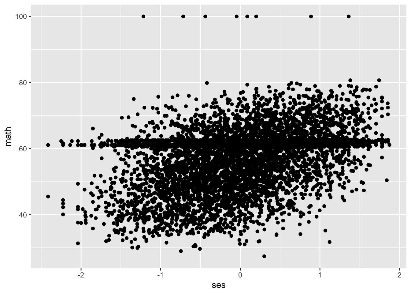
ggplot(data = data, mapping = aes(x = ses, y = math)) +
  geom_point()

Our graph reflects the positive relationship between SES and math achievement (and also shows a lot of math scores collecting around the 60 mark).

2.2.4 Multiple Regression

Next, let’s add the available sex variable female (0 = male, 1 = female) as a predictor in our regression and interpret the coefficients and R-squared value.

model2 <- lm(math ~ ses + female, data = data)
summary(model2)

## 
## Call:
## lm(formula = math ~ ses + female, data = data)
## 
## Residuals:
##     Min      1Q  Median      3Q     Max 
## -30.923  -4.606   1.176   5.317  48.054 
## 
## Coefficients:
##             Estimate Std. Error t value Pr(>|t|)    
## (Intercept)  58.1330     0.1390 418.093  < 2e-16 ***
## ses           4.2269     0.1255  33.679  < 2e-16 ***
## female       -1.0626     0.1960  -5.422 6.09e-08 ***
## ---
## Signif. codes:  0 '***' 0.001 '**' 0.01 '*' 0.05 '.' 0.1 ' ' 1
## 
## Residual standard error: 8.115 on 6868 degrees of freedom
## Multiple R-squared:  0.1467, Adjusted R-squared:  0.1464 
## F-statistic: 590.3 on 2 and 6868 DF,  p-value: < 2.2e-16

The intercept of 58.13 reflects the average math achievement score (out of 100) for male students (female = 0) at their class average SES (ses = 0). For a one-unit increase in SES, math achievement increases by 4.23 points, controlling for sex. Female students had a math achievement score lower by 1.06 points on average, controlling for SES. SES and sex together explain 14.6% of the variance in math achievement.

2.2.5 Interaction Terms

In the previous model, we assumed that the relationship between SES and math achievement was constant for both sexes (homogeneity of regression slopes, i.e., an ANCOVA model). As a final exercise, let’s add an interaction term to our regression between sex and SES.

model3 <- lm(math ~ ses + female + ses:female, data = data)
summary(model3)

## 
## Call:
## lm(formula = math ~ ses + female + ses:female, data = data)
## 
## Residuals:
##     Min      1Q  Median      3Q     Max 
## -30.975  -4.596   1.172   5.288  48.265 
## 
## Coefficients:
##             Estimate Std. Error t value Pr(>|t|)    
## (Intercept)  58.1441     0.1393 417.506  < 2e-16 ***
## ses           4.0533     0.1775  22.840  < 2e-16 ***
## female       -1.0737     0.1961  -5.475 4.54e-08 ***
## ses:female    0.3472     0.2510   1.383    0.167    
## ---
## Signif. codes:  0 '***' 0.001 '**' 0.01 '*' 0.05 '.' 0.1 ' ' 1
## 
## Residual standard error: 8.115 on 6867 degrees of freedom
## Multiple R-squared:  0.1469, Adjusted R-squared:  0.1465 
## F-statistic: 394.2 on 3 and 6867 DF,  p-value: < 2.2e-16

# Could also succinctly code it as follows:
# lm(math ~ ses*female, data = data)

An interaction captures that the relationship between two variables may differ based on the level of another variable (i.e., different slopes for different folks). An interaction term, A:B, has two possible interpretations:

The effect of A on the effect of B on your outcome Y.
The effect of B on the effect of A on your outcome Y.

The ses:female interaction term, .34, represents the effect of being female on the relationship between SES and math achievement. Alternatively, it could represent the effect of SES on the relationship between being female and math achievement. In this case, the latter is a more intuitive interpretation: female students from higher socioeconomic statuses are slightly insulated from the negative relationship between female and math achievement in this sample. As SES increases by one point, the relationship between being female and math achievement becomes less negative, from -1.07 to -.73 (-1.07 + .34). However, this interaction term is not statistically significantly different from zero per the p-value.

We can see this graphically using the sjPlot package:

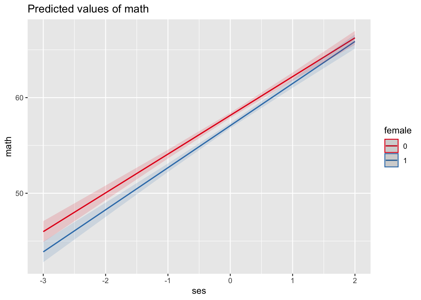
sjPlot::plot_model(model3, type = "pred", terms = c("ses", "female"))

As we can see, math scores for males (female = 0, the red line) are higher than those for females (female = 1, the blue line) at all levels of SES. However, the difference between males and females shrinks with increasing SES, as indicated by math scores at higher SES levels being closer than those at lower levels of SES.

The other coefficients have the same interpretations as before. The R-squared indicates that SES and sex account for 14.7% of the variance in math achievement.

2.3 Conclusion

If you feel comfortable with the material presented in this data demonstration, then you have a sufficiently strong baseline to move forward with the materials. In this chapter, we ignored that students were clustered into schools; in the next chapter, we’ll examine that clustering, consider its implications for our analyses, and introduce one non-multilevel-model method for handling clustered data.