Chapter 7 Model Estimation Options, Problems, and Troubleshooting
7.1 Learning Objectives
In this chapter, we will review common estimation options, problems that can arise, and how to troubleshoot those problems.
The learning objectives for this chapter are:
- Differentiate between restricted maximum likelihood and full information maximum likelihood estimation options;
- Describe common causes of estimation errors;
- Understand the components of optimizer functions;
- Recognize estimation errors in R output and examine output to identify error sources;
- Build and compare models to address errors.
All materials for this chapter are available for download here.
7.2 Data Demonstration
The data for this chapter were taken from chapter 3 of Heck, R. H., Thomas, S. L., & Tabata, L. N. (2011). Multilevel and Longitudinal Modeling with IBM SPSS: Taylor & Francis. Students are clustered within schools in the data.
7.2.1 Load Data and Dependencies
For this data demo, we will use the following packages:
library(dplyr) # for data manipulation
library(ggplot2) # for graphing
library(lme4) # for multilevel models
library(lmerTest) # for p-values
And the same dataset of students’ math achievement:
7.2.2 Introduction to Estimation Problems
In Chapter 6, we modelled the relationship between SES and math achievement with a random intercept and random slope as follows:
## boundary (singular) fit: see help('isSingular')As indicated by the warning message from R, our model is singular (which we’ll define in a moment). In this chapter, we will examine estimation issues like this and how to troubleshoot them. This is one of the less interactive chapters in these materials, but if you want a reason to stick around, there is a fun puzzle analogy. We’ll begin with some notes on model estimation and then move onto possible issues and how to address them.
7.2.3 Estimation and Optimizers
In linear regression, Ordinary Least Squares estimation is used to find a combination of parameters (intercepts and slopes) that minimize the residual sum of squares. If we imagine a simple linear regression with math achievement as an outcome and SES as a predictor, we have our regression line (line of best fit) and our actual data points around that line.
data %>%
  filter(schcode <= 10) %>% # subset data to make it easier to see
  ggplot(mapping = aes(x = ses, y = math)) +
  geom_point() +
  geom_smooth(method = "lm", se = FALSE, fullrange = TRUE)
## `geom_smooth()` using formula = 'y ~ x'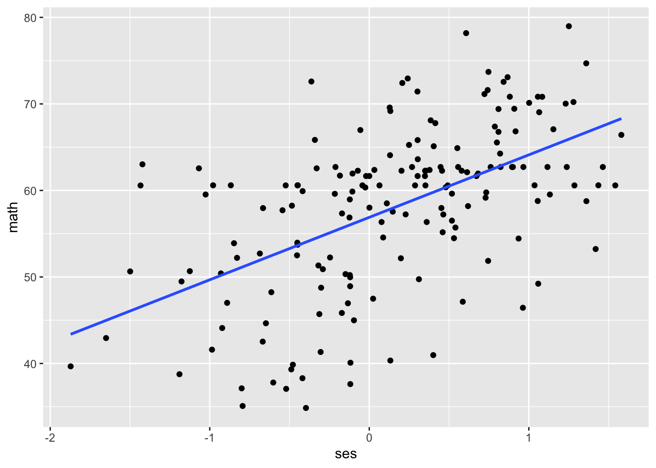
For a given value of SES on the x-axis, the distance between our prediction (regression line) and our actual observation (data point) is our residual, and if we sum all of the residuals (after squaring them so the negative residuals below the line and positive residuals above it don’t cancel out), we get our residual sum of squares. OLS regression will select the regression line with the smallest residuals, which is the line that is as close as possible to the data points. You can see this process and play around with it on this interactive website: https://seeing-theory.brown.edu/regression-analysis/index.html#section1
In multilevel modelling, we use maximum likelihood (ML) estimation instead of OLS estimation. In ML estimation, we have our data points and we want to find the combination of parameters (intercepts and slopes) that maximize the likelihood that we observed that data. This is an iterative process, where we select parameters that maximize the probability of getting our data (i.e., that maximize the likelihood). We select set after set of parameters, and eventually stop when the parameter sets aren’t getting better. You can play around with likelihood here: https://seeing-theory.brown.edu/bayesian-inference/index.html#section2 This video from Stat Quest walks through the concept:
We have two options for ML estimation in multilevel modelling: restricted maximum likelihood (REML) and full information maximum likelihood (FIML or ML). The key difference between them is how the estimation methods handle the variance components. When using REML, there is a penalty applied to the degrees of freedom when estimating the variance components \(\sigma^2\), \(\tau_1^2\), etc. When using FIML, there is no such penalty and as a result the variance components are usually underestimated. A linear regression analogy might help clarify this point: the formula for population variance is \(S = \frac{\Sigma(x_i - \overline{x})^2}{n}\). The formula for sample variance is \(s = \frac{\Sigma(x_i - \overline{x})^2}{n - 1}\). The sample variance imposes a penalty of n - 1 and is a REML estimator, while the population variance formula is the corresponding FIML estimator. Because we want accurate information about our variance components, we will usually use REML. We will only use FIML when we want to compare two models with different fixed effects. We’ll discuss model comparison later in this chapter.
7.2.4 Non-Convergence
In the embedded Stat Quest video above, the narrator describes the iterative process in ML estimation of finding the maximum likelihood estimate of a parameter, trying multiple different options before settling on one as the value that maximizes the likelihood of observing their data about mice weights. When you’re working with many predictors at once — for example, an intercept and a slope for SES and a slope for school type and variance terms for all of those fixed effects — it is harder to try all possible combinations. So, optimization algorithms (AKA optimizers) are used to try to find the ML estimates by examining a subset of possible combinations. However, these optimizers cannot always find the combination of parameters that maximizes the likelihood of observing your data; they can’t find a solution to the problem of “what paramaters maximize the likelihood of observing this data?”. When the optimizers cannot find a solution, the result is called non-convergence: the model did not converge on a solution.
You should not use the parameter estimates from a non-converged solution. A non-convergence warning is the computing equivalent of being unable to put a puzzle together, jamming the pieces in where you can, and saying “I don’t know, this is my best guess about where these pieces go.” Sure, the puzzle might sort of look like the image on the box, but it doesn’t really match, a bunch of the pieces have been contorted and bent to fit.
There are two main strategies to solve a non-convergence problem: change your optimizer or change your model. You can manipulate a few characteristics of your optimizer to try to get convergence:
- Number of iterations. If you increase the number of iterations, the algorithm will search for longer. This is the equivalent of getting our puzzle-doer to sit at the table for longer trying to assemble the puzzle, trying out different and more pieces.
- Algorithm: the algorithm determines how the optimizer chooses its next attempted solution. What strategy is our puzzle-doer using to fit pieces into the puzzle?
- Tolerance: this can get a bit technical and vary depending on context, so we suggest Brauer and Curtin, 2018 for more. But in our case, we can think of it as the algorithm’s tolerance for differences in solutions. Lower tolerance means slightly different solutions will be seen as different, whereas higher tolerance means two different solutions that are still kind of close will be treated as essentially the same. Maybe our puzzle-doer needs glasses; tolerance is like whether they’re wearing their glasses and can distinguish between two close-but-not-identical assembled puzzles.
(We hope you enjoyed the puzzle analogy.)
You can alter these elements of your optimizer to see if giving it more time, a different strategy, or more leeway to say “yes, this converged” will lead to convergence. Alternatively, you can trim your model, removing variables you think are less likely to matter. We will discuss some approaches to doing this below.
7.2.5 Singularity
Singularity occurs when an element of your variance-covariance matrix is estimated as essentially zero as a result of extreme multicollinearity or because the parameter is actually essentially zero.
You can find singularity by examining your variance-covariance estimates and the correlations between them. It will often show up as co/variances near zero or correlations between variances at -1 or 1. Let’s return to our example from Chapter 6, predicting math achievement from SES with a random slope:
## boundary (singular) fit: see help('isSingular')As we can see, our output contains a helpful warning message notifying us that the model is singular. We can investigate this issue in three ways. First, we can look at our Tau matrix:
## 2 x 2 sparse Matrix of class "dsCMatrix"
##             (Intercept)        ses
## (Intercept)    3.204184 -1.5802590
## ses           -1.580259  0.7793617
Things look okay here, no elements appear to be close to or zero. Our second method of investigation is looking at our overall output:
## Linear mixed model fit by REML. t-tests use Satterthwaite's method ['lmerModLmerTest']
## Formula: math ~ 1 + ses + (1 + ses | schcode)
##    Data: data
##
## REML criterion at convergence: 48190.1
##
## Scaled residuals:
##     Min      1Q  Median      3Q     Max
## -3.8578 -0.5553  0.1290  0.6437  5.7098
##
## Random effects:
##  Groups   Name        Variance Std.Dev. Corr
##  schcode  (Intercept)  3.2042  1.7900
##           ses          0.7794  0.8828   -1.00
##  Residual             62.5855  7.9111
## Number of obs: 6871, groups:  schcode, 419
##
## Fixed effects:
##              Estimate Std. Error        df t value Pr(>|t|)
## (Intercept)   57.6959     0.1315  378.6378  438.78   <2e-16 ***
## ses            3.9602     0.1408 1450.7730   28.12   <2e-16 ***
## ---
## Signif. codes:  0 '***' 0.001 '**' 0.01 '*' 0.05 '.' 0.1 ' ' 1
##
## Correlation of Fixed Effects:
##     (Intr)
## ses -0.284
## optimizer (nloptwrap) convergence code: 0 (OK)
## boundary (singular) fit: see help('isSingular')
Here, in our random effects section, we can see that the correlation between our random effect variances is -1.00, a sign of perfect multicollinearity. We can dig into the confidence intervals of our estimates up close to confirm this:
## Computing profile confidence intervals ...## 2.5 % 97.5 %
## sd_(Intercept)|schcode 1.4999340 2.0751034
## cor_ses.(Intercept)|schcode -1.0000000 -0.6587309
## sd_ses|schcode 0.5410211 1.2341712
## sigma 7.7773576 8.0484788
## (Intercept) 57.4380811 57.9532857
## ses 3.6737845 4.2507467Note that oldNames = FALSE just makes the output easier to read. This will take a moment to run, but when it does we can see that the 95% confidence interval for the correlation between our random effect variances spans -1 to 1 (i.e. the entire possible range). Our singularity issue started when we added the random slope effect, which added both a random slope variance \(\tau_1^2\) and the random intercept-slope covariance \(\tau_{01}\). Let’s see if we can fix the issue by removing that problematic covariance.
ses_l1_random_cov0 <- lmer(math ~ 1 + ses + (1|schcode) + (0 + ses|schcode), data = data, REML = TRUE)
summary(ses_l1_random_cov0)
## Linear mixed model fit by REML. t-tests use Satterthwaite's method ['lmerModLmerTest']
## Formula: math ~ 1 + ses + (1 | schcode) + (0 + ses | schcode)
## Data: data
##
## REML criterion at convergence: 48213.4
##
## Scaled residuals:
## Min 1Q Median 3Q Max
## -3.7791 -0.5526 0.1327 0.6466 5.7089
##
## Random effects:
## Groups Name Variance Std.Dev.
## schcode (Intercept) 3.3222 1.8227
## schcode.1 ses 0.7205 0.8488
## Residual 62.5213 7.9070
## Number of obs: 6871, groups: schcode, 419
##
## Fixed effects:
## Estimate Std. Error df t value Pr(>|t|)
## (Intercept) 57.5888 0.1328 374.9738 433.55 <2e-16 ***
## ses 3.8803 0.1435 377.2408 27.04 <2e-16 ***
## ---
## Signif. codes: 0 '***' 0.001 '**' 0.01 '*' 0.05 '.' 0.1 ' ' 1
##
## Correlation of Fixed Effects:
## (Intr)
## ses -0.023Here, we specify our random intercept (1|schcode) and random slope with no covariance (0 + ses|schcode) separately, and that fixed the singularity issue! If we print our Tau matrix we can see that the covariance is fixed to 0.
## 2 x 2 sparse Matrix of class "dsCMatrix"
##
## [1,] 3.322166 .
## [2,] .        0.7204535
In general, it is best practice to build a maximal multilevel model, one that includes all possible fixed and random effects that are not zero (Barr et al., 2013). This maximal model will produce parameter estimates with the least amount of bias and provide the best shot at your model fitting the data. However, the maximal model that tries to estimate extreme random effect variances (those near zero or with high multicollinearity) will have trouble converging and produce estimation errors. When this happens, often an inspection of the random effect variances will reveal which parameters need to be removed from the model. It can be helpful, ahead of running your MLMs, to consider the key variables of interest, their random effects, and plan, if the maximal model has errors, which parameters should be removed and in what order. Overall, building MLMs is about balancing complexity with utility. Sometimes we do not have enough information in our data to estimate the complex model we planned, so having a plan for how to decrease complexity ahead of time can prevent getting lost in the garden of forking paths.
7.2.6 Deviance Testing for Model Comparison
We removed the random effect covariance and our model is no longer singular (i.e., suffering from multicollinearity). That seems better! Now that we have a model without an error, let’s look at comparing the model with the random slope for SES (but no covariance, as we just removed that) and the model without the random slope for SES. If we want to formally test if a model fit is better or at least not worse, we can conduct a deviance test. You can find the “deviance” for your model under the “REML criterion at convergence” in your summary output. In short, deviance is bad and we don’t want more of it, so when we compare the model with and without the random slope for SES, we don’t want the model with the random slope to have more deviance. We want the same or less deviance.
Note that deviance is based on the likelihood function for your model. Unlike probability, likelihood is not bound at 0 and 1. It can be any number. As a result, looking at likelihood or deviance in isolation is not informative, because it has no bounds. It is only useful for comparison between models, where less deviance indicates a better model (compared to the reference model).
Here, we’re comparing models with the same fixed effects but different random effects so we can still use REML estimator that more accurately estimates random effects. We have our two model terms, ses_l1 and ses_l1_random_cov0, and we can compare the deviance of each using the built-in ANOVA function. Specifying refit = FALSE stops the function from refitting the models with FIML. If we were comparing models with different fixed effects, we would use FIML to estimate our models.
# models
ses_l1 <- lmer(math ~ 1 + ses + (1|schcode), data = data, REML = TRUE)
ses_l1_random_cov0 <- lmer(math ~ 1 + ses + (1|schcode) + (0 + ses|schcode), data = data, REML = TRUE)

# deviance test to compare model fit
anova(ses_l1, ses_l1_random_cov0, refit = FALSE)
## Data: data
## Models:
## ses_l1: math ~ 1 + ses + (1 | schcode)
## ses_l1_random_cov0: math ~ 1 + ses + (1 | schcode) + (0 + ses | schcode)
## npar AIC BIC logLik deviance Chisq Df Pr(>Chisq)
## ses_l1 4 48223 48251 -24108 48215
## ses_l1_random_cov0 5 48223 48258 -24107 48213 2.0825 1 0.149Let’s read our output. We have seven columns:
- npar is the number of parameters estimated in the models. The only difference between the models is one has a random slope for SES and the other doesn’t, and you can see that one model estimates 4 parameters and the other 5 parameters.
- AIC: Akaike’s Information Criterion, one measure of goodness of fit
- BIC: Bayesian Information Criterion, another measure of goodness of fit
- logLik: log likelihood
- deviance: -2*logLik
- Chisq: the difference betwen our models’ deviances
- df: the degrees of freedom for the test, calculated as the difference in number of parameters between the models
- Pr(>Chisq): the probability that we would find our chi-square value or greater if the null hypothesis that the models were the same was true
There is no significant difference between our models’ deviance statistics: the model without the random slope has a deviance of 48215 and the model with the covariance has a deviance of 48213. The difference between these numbers is not significant, p = 0.149. Thus, there is no significant different in model fits and adding a random slope does not compromise model fit so we can add it if we think it’s informative.
We’ll discuss model specification, fit, and comparison more in Chapter 11 when discussing effect sizes. In closing, when assessing model fit or troubleshooting estimation problems, it is preferable to pre-register what troubleshooting you expect to try or models you expect to estimate. At minimum, you should keep a record of changes you make and report all of them.
7.3 Conclusion
In this chapter, we considered convergence options, how to diagnose and troubleshoot issues, and comparing model fits using deviance testing. In Chapter 8, we’ll consider different centering options in MLMs.
7.4 Further Reading
Barr, D. J., Levy, R., Scheepers, C., & Tily, H. J. (2013). Random effects structure for confirmatory hypothesis testing: Keep it maximal. Journal of memory and language, 68(3), 10.1016/j.jml.2012.11.001. https://doi.org/10.1016/j.jml.2012.11.001
Brauer, M., & Curtin, J. J. (2018). Linear mixed-effects models and the analysis of nonindependent data: A unified framework to analyze categorical and continuous independent variables that vary within-subjects and/or within-items. Psychological Methods, 23(3), 389–411.